6 6 | THE NORMAL DISTRIBUTION

Figure 6.1 If you ask enough people about their shoe size, you will find that your graphed data is shaped like a bell curve and can be described as normally distributed. (credit: Ömer Ünlϋ)

Introduction

The normal probability density function, a continuous distribution, is the most important of all the distributions. It is widely used and even more widely abused. Its graph is bell-shaped. You see the bell curve in almost all disciplines. Some of these include psychology, business, economics, the sciences, nursing, and, of course, mathematics. Some of your instructors may use the normal distribution to help determine your grade. Most IQ scores are normally distributed. Often real-estate prices fit a normal distribution.

The normal distribution is extremely important, but it cannot be applied to everything in the real world. Remember here that we are still talking about the distribution of population data. This is a discussion of probability and thus it is the population data that may be normally distributed, and if it is, then this is how we can find probabilities of specific events just as we did for population data that may be binomially distributed or Poisson distributed. This caution is here because in the next chapter we will see that the normal distribution describes something very different from raw data and forms the foundation of inferential statistics.

The normal distribution has two parameters (two numerical descriptive measures): the mean (μ) and the standard deviation (σ). If X is a quantity to be measured that has a normal distribution with mean (μ) and standard deviation (σ), we designate this by writing the following formula of the normal probability density function:

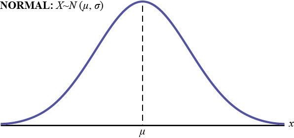
Figure 6.2

The probability density function is a rather complicated function. Do not memorize it. It is not necessary.

− 1 ⋅ ⎛x − µ ⎞2

f (x) = 1⋅ e 2 ⎝ σ ⎠

σ ⋅ 2 ⋅ π

The curve is symmetric about a vertical line drawn through the mean, μ. The mean is the same as the median, which is the same as the mode, because the graph is symmetric about μ. As the notation indicates, the normal distribution depends only on the mean and the standard deviation. Note that this is unlike several probability density functions we have already

studied, such as the Poisson, where the mean is equal to µ and the standard deviation simply the square root of the mean, or

the binomial, where p is used to determine both the mean and standard deviation. Since the area under the curve must equal one, a change in the standard deviation, σ, causes a change in the shape of the normal curve; the curve becomes fatter and wider or skinnier and taller depending on σ. A change in μ causes the graph to shift to the left or right. This means there are an infinite number of normal probability distributions. One of special interest is called the standard normal distribution.

| The Standard Normal Distribution

The standard normal distribution is a normal distribution of standardized values called z-scores. A z-score is measured in units of the standard deviation.

The mean for the standard normal distribution is zero, and the standard deviation is one. What this does is dramatically simplify the mathematical calculation of probabilities. Take a moment and substitute zero and one in the appropriate places in the above formula and you can see that the equation collapses into one that can be much more easily solved using integral

σ
calculus. The transformation z = x − µ produces the distribution Z ~ N(0, 1). The value x in the given equation comes from

a known normal distribution with known mean μ and known standard deviation σ. The z-score tells how many standard deviations a particular x is away from the mean.

• cores

If X is a normally distributed random variable and X ~ N(μ, σ), then the z-score for a particular x is:

σ
z = x – µ

The z-score tells you how many standard deviations the value x is above (to the right of) or below (to the left of) the mean, μ. Values of x that are larger than the mean have positive z-scores, and values of x that are smaller than the mean have negative z-scores. If x equals the mean, then x has a z-score of zero.

Example 6.1Suppose X ~ N(5, 6). This says that X is a normally distributed random variable with mean μ = 5 and standard deviation σ = 6. Suppose x = 17. Then:

This OpenStax book is available for free at http://cnx.org/content/col11776/1.33

z = x – µ = 17 – 5 = 2

σ6

This means that x = 17 is two standard deviations (2σ) above or to the right of the mean μ = 5.

σ
Now suppose x = 1. Then: z = x – µ

= 1 – 5

6

= –0.67 (rounded to two decimal places)

This means that x = 1 is 0.67 standard deviations (–0.67σ) below or to the left of the mean μ = 5.

The Empirical Rule

If X is a random variable and has a normal distribution with mean µ and standard deviation σ, then the Empirical Rule

states the following:

• About 68% of the x values lie between –1σ and +1σ of the mean µ (within one standard deviation of the mean).
• About 95% of the x values lie between –2σ and +2σ of the mean µ (within two standard deviations of the mean).
• About 99.7% of the x values lie between –3σ and +3σ of the mean µ (within three standard deviations of the mean). Notice that almost all the x values lie within three standard deviations of the mean.
• The z-scores for +1σ and –1σ are +1 and –1, respectively.
• The z-scores for +2σ and –2σ are +2 and –2, respectively.
• The z-scores for +3σ and –3σ are +3 and –3 respectively.

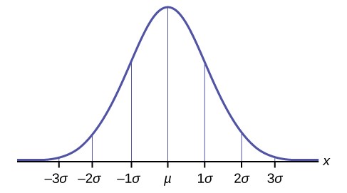
Figure 6.3

Example 6.2Suppose x has a normal distribution with mean 50 and standard deviation 6.About 68% of the x values lie within one standard deviation of the mean. Therefore, about 68% of the x values lie between –1σ = (–1)(6) = –6 and 1σ = (1)(6) = 6 of the mean 50. The values 50 – 6 = 44 and 50+ 6 = 56 are within one standard deviation from the mean 50. The z-scores are –1 and +1 for 44 and 56, respectively.About 95% of the x values lie within two standard deviations of the mean. Therefore, about 95% of the x values lie between –2σ = (–2)(6) = –12 and 2σ = (2)(6) = 12. The values 50 – 12 = 38 and 50 + 12 = 62 are within two standard deviations from the mean 50. The z-scores are –2 and +2 for 38 and 62, respectively.About 99.7% of the x values lie within three standard deviations of the mean. Therefore, about 95% of the x values lie between –3σ = (–3)(6) = –18 and 3σ = (3)(6) = 18 of the mean 50. The values 50 – 18 = 32 and 50+ 18 = 68 are within three standard deviations from the mean 50. The z-scores are –3 and +3 for 32 and 68, respectively.

| Using the Normal Distribution

The shaded area in the following graph indicates the area to the right of x. This area is represented by the probability P(X > x). Normal tables provide the probability between the mean, zero for the standard normal distribution, and a specific value such as x1 . This is the unshaded part of the graph from the mean to x1 .

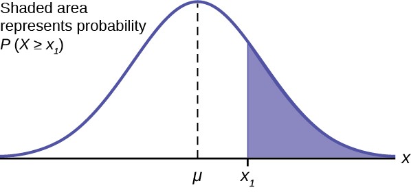
Figure 6.4

Because the normal distribution is symmetrical , if x1 were the same distance to the left of the mean the area, probability, in the left tail, would be the same as the shaded area in the right tail. Also, bear in mind that because of the symmetry of this distribution, one-half of the probability is to the right of the mean and one-half is to the left of the mean.

Calculations of Probabilities

To find the probability for probability density functions with a continuous random variable we need to calculate the area under the function across the values of X we are interested in. For the normal distribution this seems a difficult task given the complexity of the formula. There is, however, a simply way to get what we want. Here again is the formula for the normal distribution:

− 1 ⋅ ⎛x − µ ⎞2

f (x) = 1⋅ e 2 ⎝ σ ⎠

σ ⋅ 2 ⋅ π

Looking at the formula for the normal distribution it is not clear just how we are going to solve for the probability doing it the same way we did it with the previous probability functions. There we put the data into the formula and did the math.

To solve this puzzle we start knowing that the area under a probability density function is the probability.

This OpenStax book is available for free at http://cnx.org/content/col11776/1.33

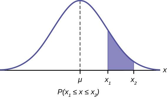
Figure 6.5

This shows that the area between X1 and X2 is the probability as stated in the formula: P (X1 ≤ x ≤ X2)

The mathematical tool needed to find the area under a curve is integral calculus. The integral of the normal probability density function between the two points x1 and x2 is the area under the curve between these two points and is the probability between these two points.

Doing these integrals is no fun and can be very time consuming. But now, remembering that there are an infinite number of normal distributions out there, we can consider the one with a mean of zero and a standard deviation of 1. This particular normal distribution is given the name Standard Normal Distribution. Putting these values into the formula it reduces to a very simple equation. We can now quite easily calculate all probabilities for any value of x, for this particular normal distribution, that has a mean of zero and a standard deviation of 1. These have been produced and are available here in the appendix to the text or everywhere on the web. They are presented in various ways. The table in this text is the most common presentation and is set up with probabilities for one-half the distribution beginning with zero, the mean, and moving outward. The shaded area in the graph at the top of the table in Statistical Tables represents the probability from zero to the specific Z value noted on the horizontal axis, Z.

The only problem is that even with this table, it would be a ridiculous coincidence that our data had a mean of zero and a standard deviation of one. The solution is to convert the distribution we have with its mean and standard deviation to this new Standard Normal Distribution. The Standard Normal has a random variable called Z.

Using the standard normal table, typically called the normal table, to find the probability of one standard deviation, go to the Z column, reading down to 1.0 and then read at column 0. That number, 0.3413 is the probability from zero to 1 standard deviation. At the top of the table is the shaded area in the distribution which is the probability for one standard deviation. The table has solved our integral calculus problem. But only if our data has a mean of zero and a standard deviation of 1.

However, the essential point here is, the probability for one standard deviation on one normal distribution is the same on every normal distribution. If the population data set has a mean of 10 and a standard deviation of 5 then the probability from 10 to 15, one standard deviation, is the same as from zero to 1, one standard deviation on the standard normal distribution. To compute probabilities, areas, for any normal distribution, we need only to convert the particular normal distribution to the standard normal distribution and look up the answer in the tables. As review, here again is the standardizing formula:

σ
Z = x – µ

where Z is the value on the standard normal distribution, X is the value from a normal distribution one wishes to convert to the standard normal, μ and σ are, respectively, the mean and standard deviation of that population. Note that the equation uses μ and σ which denotes population parameters. This is still dealing with probability so we always are dealing with the population, with known parameter values and a known distribution. It is also important to note that because the normal distribution is symmetrical it does not matter if the z-score is positive or negative when calculating a probability. One standard deviation to the left (negative Z-score) covers the same area as one standard deviation to the right (positive Z- score). This fact is why the Standard Normal tables do not provide areas for the left side of the distribution. Because of this symmetry, the Z-score formula is sometimes written as:

σ
Z = |x – µ|

Where the vertical lines in the equation means the absolute value of the number.

What the standardizing formula is really doing is computing the number of standard deviations X is from the mean of its own distribution. The standardizing formula and the concept of counting standard deviations from the mean is the secret of all that we will do in this statistics class. The reason this is true is that all of statistics boils down to variation, and the counting of standard deviations is a measure of variation.

This formula, in many disguises, will reappear over and over throughout this course.

Example 6.3

The final exam scores in a statistics class were normally distributed with a mean of 63 and a standard deviation of five.

• Find the probability that a randomly selected student scored more than 65 on the exam.
• Find the probability that a randomly selected student scored less than 85.

Solution 6.3

• Let X = a score on the final exam. X ~ N(63, 5), where μ = 63 and σ = 5. Draw a graph.

Then, find P(x > 65).

P(x > 65) = 0.3446

Figure 6.6

Z1 = x1 − µ = 65 − 63 = 0.4

σ5

This OpenStax book is available for free at http://cnx.org/content/col11776/1.33

P(x ≥ x1) = P(Z ≥ Z1) = 0.3446

The probability that any student selected at random scores more than 65 is 0.3446. Here is how we found this answer.

The normal table provides probabilities from zero to the value Z1. For this problem the question can be written as: P(X ≥ 65) = P(Z ≥ Z1), which is the area in the tail. To find this area the formula would be 0.5 – P(X ≤ 65). One half of the probability is above the mean value because this is a symmetrical distribution. The graph shows how to find the area in the tail by subtracting that portion from the mean, zero, to the Z1 value. The final answer is: P(X ≥ 63) = P(Z ≥ 0.4) = 0.3446

z = 65 – 63

5

= 0.4

Area to the left of Z1 to the mean of zero is 0.1554

P(x > 65) = P(z > 0.4) = 0.5 – 0.1554 = 0.3446

Solution 6.3

b.

Z = x – µ = 85 – 63 = 4.4 which is larger than the maximum value on the Standard Normal Table. Therefore,

σ5

the probability that one student scores less than 85 is approximately one or 100%.

A score of 85 is 4.4 standard deviations from the mean of 63 which is beyond the range of the standard normal table. Therefore, the probability that one student scores less than 85 is approximately one (or 100%).

6.3 The golf scores for a school team were normally distributed with a mean of 68 and a standard deviation of three. Find the probability that a randomly selected golfer scored less than 65.
Example 6.4A personal computer is used for office work at home, research, communication, personal finances, education, entertainment, social networking, and a myriad of other things. Suppose that the average number of hours a household personal computer is used for entertainment is two hours per day. Assume the times for entertainment are normally distributed and the standard deviation for the times is half an hour.a. Find the probability that a household personal computer is used for entertainment between 1.8 and 2.75 hours per day.Solution 6.4a. Let X = the amount of time (in hours) a household personal computer is used for entertainment. X ~ N(2, 0.5) where μ = 2 and σ = 0.5.Find P(1.8 < x < 2.75).The probability for which you are looking is the area between x = 1.8 and x = 2.75. P(1.8 < x < 2.75) = 0.5886

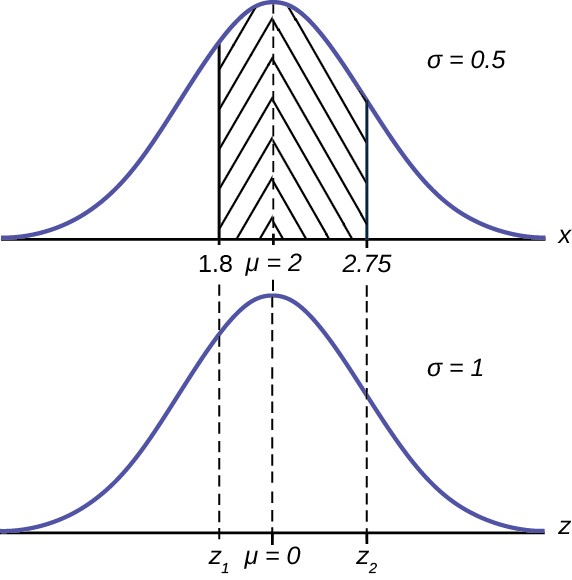
Figure 6.7

P(1.8 ≤ x ≤ 2.75) = P(Zi ≤ Z ≤ Z2)

The probability that a household personal computer is used between 1.8 and 2.75 hours per day for entertainment is 0.5886.

• Find the maximum number of hours per day that the bottom quartile of households uses a personal computer for entertainment.

Solution 6.4

b. To find the maximum number of hours per day that the bottom quartile of households uses a personal computer for entertainment, find the 25th percentile, k, where P(x < k) = 0.25.

This OpenStax book is available for free at http://cnx.org/content/col11776/1.33

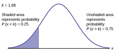
Figure 6.8

f ⎛Z⎞ = 0.5 – 0.25 = 0.25 , therefore Z ≈ -0.675 (or just 0.67 using the table) Z = x – µ = x – 2 = -0.675 ,

⎝ ⎠σ

0.5

therefore x = -0.675 * 0.5 + 2 = 1.66 hours.

The maximum number of hours per day that the bottom quartile of households uses a personal computer for entertainment is 1.66 hours.

6.4 The golf scores for a school team were normally distributed with a mean of 68 and a standard deviation of three. Find the probability that a golfer scored between 66 and 70.
Example 6.5In the United States the ages 13 to 55+ of smartphone users approximately follow a normal distribution with approximate mean and standard deviation of 36.9 years and 13.9 years, respectively.Determine the probability that a random smartphone user in the age range 13 to 55+ is between 23 and 64.7 years old.Solution 6.5a. 0.8186Determine the probability that a randomly selected smartphone user in the age range 13 to 55+ is at most 50.8 years old.Solution 6.5b. 0.8413

Example 6.6

A citrus farmer who grows mandarin oranges finds that the diameters of mandarin oranges harvested on his farm follow a normal distribution with a mean diameter of 5.85 cm and a standard deviation of 0.24 cm.

• Find the probability that a randomly selected mandarin orange from this farm has a diameter larger than 6.0 cm. Sketch the graph.

Solution 6.6

Figure 6.9

P(x ≥ 6) = P(z ≥ 0.625) = 0.2670

Z1 = 6 − 5.85 = .625

• .24
  The middle 20% of mandarin oranges from this farm have diameters between and .

Solution 6.6

f ⎛Z⎞ = 0.20 = 0.10 , therefore Z ≈ ± 0.25

⎝ ⎠2

Z = x – µ = x – 5.85 = ± 0.25 → ± 0.25 * 0.24 + 5.85 = ⎛5.79, 5.91⎞

σ0.24⎝⎠

This OpenStax book is available for free at http://cnx.org/content/col11776/1.33

| Estimating the Binomial with the Normal Distribution

We found earlier that various probability density functions are the limiting distributions of others; thus, we can estimate one with another under certain circumstances. We will find here that the normal distribution can be used to estimate a binomial process. The Poisson was used to estimate the binomial previously, and the binomial was used to estimate the hypergeometric distribution.

In the case of the relationship between the hypergeometric distribution and the binomial, we had to recognize that a binomial process assumes that the probability of a success remains constant from trial to trial: a head on the last flip cannot have an effect on the probability of a head on the next flip. In the hypergeometric distribution this is the essence of the question because the experiment assumes that any “draw” is without replacement. If one draws without replacement, then all subsequent “draws” are conditional probabilities. We found that if the hypergeometric experiment draws only a small percentage of the total objects, then we can ignore the impact on the probability from draw to draw.

Imagine that there are 312 cards in a deck comprised of 6 normal decks. If the experiment called for drawing only 10 cards, less than 5% of the total, than we will accept the binomial estimate of the probability, even though this is actually a hypergeometric distribution because the cards are presumably drawn without replacement.

The Poisson likewise was considered an appropriate estimate of the binomial under certain circumstances. In Chapter 4

we found that if the number of trials of interest is large and the probability of success is small, such that µ = np < 7 , the

Poisson can be used to estimate the binomial with good results. Again, these rules of thumb do not in any way claim that the actual probability is what the estimate determines, only that the difference is in the third or fourth decimal and is thus de minimus.

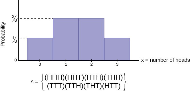
Here, again, we find that the normal distribution makes particularly accurate estimates of a binomial process under certain circumstances. Figure 6.10 is a frequency distribution of a binomial process for the experiment of flipping three coins where the random variable is the number of heads. The sample space is listed below the distribution. The experiment assumed that the probability of a success is 0.5; the probability of a failure, a tail, is thus also 0.5. In observing Figure 6.10 we are struck by the fact that the distribution is symmetrical. The root of this result is that the probabilities of success and failure are the same, 0.5. If the probability of success were smaller than 0.5, the distribution becomes skewed right. Indeed, as the probability of success diminishes, the degree of skewness increases. If the probability of success increases from 0.5, then the skewness increases in the lower tail, resulting in a left-skewed distribution.

Figure 6.10

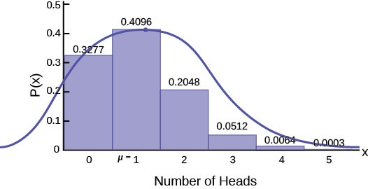
The reason the skewness of the binomial distribution is important is because if it is to be estimated with a normal distribution, then we need to recognize that the normal distribution is symmetrical. The closer the underlying binomial distribution is to being symmetrical, the better the estimate that is produced by the normal distribution. Figure 6.11 shows a symmetrical normal distribution transposed on a graph of a binomial distribution where p = 0.2 and n = 5. The discrepancy

between the estimated probability using a normal distribution and the probability of the original binomial distribution is apparent. The criteria for using a normal distribution to estimate a binomial thus addresses this problem by requiring BOTH np AND n(1 − p) are greater than five. Again, this is a rule of thumb, but is effective and results in acceptable estimates of the binomial probability.

Figure 6.11

Example 6.7

Imagine that it is known that only 10% of Australian Shepherd puppies are born with what is called “perfect symmetry” in their three colors, black, white, and copper. Perfect symmetry is defined as equal coverage on all parts of the dog when looked at in the face and measuring left and right down the centerline. A kennel would have a good reputation for breeding Australian Shepherds if they had a high percentage of dogs that met this criterion. During the past 5 years and out of the 100 dogs born to Dundee Kennels, 16 were born with this coloring characteristic.

What is the probability that, in 100 births, more than 16 would have this characteristic?

Solution 6.7

If we assume that one dog’s coloring is independent of other dogs’ coloring, a bit of a brave assumption, this becomes a classic binomial probability problem.

The statement of the probability requested is 1 − [p(X = 0) + p(X = 1) + p(X = 2)+ … + p(X = 16)]. This requires us to calculate 17 binomial formulas and add them together and then subtract from one to get the right hand part of the distribution. Alternatively, we can use the normal distribution to get an acceptable answer and in much less time.

First, we need to check if the binomial distribution is symmetrical enough to use the normal distribution. We know that the binomial for this problem is skewed because the probability of success, 0.1, is not the same as the

probability of failure, 0.9. Nevertheless, both np = 10 and n⎛1 − p⎞ = 90 are larger than 5, the cutoff for using

⎝⎠

the normal distribution to estimate the binomial.

Figure 6.11 below shows the binomial distribution and marks the area we wish to know. The mean of the binomial, 10, is also marked, and the standard deviation is written on the side of the graph: σ = npq = 3.

The area under the distribution from zero to 16 is the probability requested, and has been shaded in. Below the binomial distribution is a normal distribution to be used to estimate this probability. That probability has also been shaded.

This OpenStax book is available for free at http://cnx.org/content/col11776/1.33

Figure 6.12

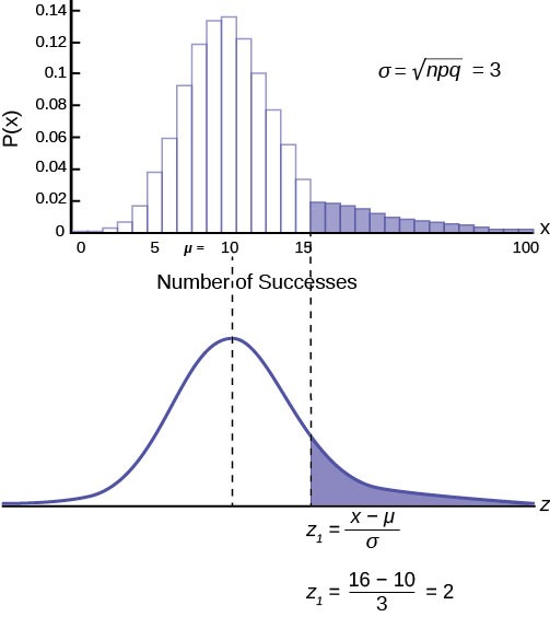
Standardizing from the binomial to the normal distribution as done in the past shows where we are asking for the probability from 16 to positive infinity, or 100 in this case. We need to calculate the number of standard deviations 16 is away from the mean: 10.

Z = x − µ = 16 − 10 = 2

σ3

We are asking for the probability beyond two standard deviations, a very unlikely event. We look up two standard deviations in the standard normal table and find the area from zero to two standard deviations is 0.4772. We are interested in the tail, however, so we subtract 0.4772 from 0.5 and thus find the area in the tail. Our conclusion is the probability of a kennel having 16 dogs with “perfect symmetry” is 0.0228. Dundee Kennels has an extraordinary record in this regard.

Mathematically, we write this as:

⎣
⎝
⎠
⎝
⎠
⎝
⎠
⎝
⎠⎦
⎝
⎠
⎝
⎠
1 − ⎡ p⎛X = 0⎞ + p⎛X = 1⎞ + p⎛X = 2⎞ + … + p⎛X = 16⎞⎤ = p⎛X > 16⎞ = p⎛Z > 2⎞ = 0.0228

KEY TERMS

Normal Distribution

a continuous random variable (RV) with pdf f(x) = 1 e

σ 2π

– (x – µ) 2 2σ 2

, where μ is the mean of

the distribution and σ is the standard deviation; notation: X ~ N(μ, σ). If μ = 0 and σ = 1, the RV, Z, is called the

standard normal distribution.

Standard Normal Distribution a continuous random variable (RV) X ~ N(0, 1); when X follows the standard normal distribution, it is often noted as Z ~ N(0, 1).

σ
σ
z-score the linear transformation of the form z = x – µ or written as z = |x – µ| ; if this transformation is applied to

any normal distribution X ~ N(μ, σ) the result is the standard normal distribution Z ~ N(0,1). If this transformation is applied to any specific value x of the RV with mean μ and standard deviation σ, the result is called the z-score of x. The z-score allows us to compare data that are normally distributed but scaled differently. A z-score is the number of standard deviations a particular x is away from its mean value.

CHAPTER REVIEW

6.1 The Standard Normal Distribution

A z-score is a standardized value. Its distribution is the standard normal, Z ~ N(0, 1). The mean of the z-scores is zero and the standard deviation is one. If z is the z-score for a value x from the normal distribution N(µ, σ) then z tells you how many standard deviations x is above (greater than) or below (less than) µ.

6.3 Estimating the Binomial with the Normal Distribution

The normal distribution, which is continuous, is the most important of all the probability distributions. Its graph is bell- shaped. This bell-shaped curve is used in almost all disciplines. Since it is a continuous distribution, the total area under the curve is one. The parameters of the normal are the mean µ and the standard deviation σ. A special normal distribution, called the standard normal distribution is the distribution of z-scores. Its mean is zero, and its standard deviation is one.

FORMULA REVIEW

6.0 Introduction

z-score: z = x – µ

σ
or z = |x – µ|

σ
X ∼ N(μ, σ)

μ = the mean; σ = the standard deviation

6.1 The Standard Normal Distribution

Z ~ N(0, 1)

z = a standardized value (z-score) mean = 0; standard deviation = 1

To find the kth percentile of X when the z-scores is known:

k = μ + (z)σ

PRACTICE

Z = the random variable for z-scores Z ~ N(0, 1)

6.3 Estimating the Binomial with the Normal Distribution

Normal Distribution: X ~ N(µ, σ) where µ is the mean and

o is the standard deviation.

Standard Normal Distribution: Z ~ N(0, 1).

This OpenStax book is available for free at http://cnx.org/content/col11776/1.33

6.1 The Standard Normal Distribution

• A bottle of water contains 12.05 fluid ounces with a standard deviation of 0.01 ounces. Define the random variable X in words. X = .
• A normal distribution has a mean of 61 and a standard deviation of 15. What is the median?

3. X ~ N(1, 2)

σ =

4. A company manufactures rubber balls. The mean diameter of a ball is 12 cm with a standard deviation of 0.2 cm. Define the random variable X in words. X = .

5. X ~ N(–4, 1)

What is the median?

6. X ~ N(3, 5)

σ =

7. X ~ N(–2, 1)

μ =

• What does a z-score measure?
• What does standardizing a normal distribution do to the mean?
• Is X ~ N(0, 1) a standardized normal distribution? Why or why not?
• What is the z-score of x = 12, if it is two standard deviations to the right of the mean?
• What is the z-score of x = 9, if it is 1.5 standard deviations to the left of the mean?
• What is the z-score of x = –2, if it is 2.78 standard deviations to the right of the mean?
• What is the z-score of x = 7, if it is 0.133 standard deviations to the left of the mean?
• Suppose X ~ N(2, 6). What value of x has a z-score of three?
• Suppose X ~ N(8, 1). What value of x has a z-score of –2.25?
• Suppose X ~ N(9, 5). What value of x has a z-score of –0.5?
• Suppose X ~ N(2, 3). What value of x has a z-score of –0.67?
• Suppose X ~ N(4, 2). What value of x is 1.5 standard deviations to the left of the mean?
• Suppose X ~ N(4, 2). What value of x is two standard deviations to the right of the mean?
• Suppose X ~ N(8, 9). What value of x is 0.67 standard deviations to the left of the mean?
• Suppose X ~ N(–1, 2). What is the z-score of x = 2?
• Suppose X ~ N(12, 6). What is the z-score of x = 2?
• Suppose X ~ N(9, 3). What is the z-score of x = 9?
• Suppose a normal distribution has a mean of six and a standard deviation of 1.5. What is the z-score of x = 5.5?
• In a normal distribution, x = 5 and z = –1.25. This tells you that x = 5 is standard deviations to the (right or left) of the mean.
• In a normal distribution, x = 3 and z = 0.67. This tells you that x = 3 is standard deviations to the (right or left) of the mean.
• In a normal distribution, x = –2 and z = 6. This tells you that x = –2 is standard deviations to the (right or left) of the mean.
• In a normal distribution, x = –5 and z = –3.14. This tells you that x = –5 is standard deviations to the (right or left) of the mean.
• In a normal distribution, x = 6 and z = –1.7. This tells you that x = 6 is standard deviations to the (right or left) of the mean.

• About what percent of x values from a normal distribution lie within one standard deviation (left and right) of the mean of that distribution?
• About what percent of the x values from a normal distribution lie within two standard deviations (left and right) of the mean of that distribution?
• About what percent of x values lie between the second and third standard deviations (both sides)?
• Suppose X ~ N(15, 3). Between what x values does 68.27% of the data lie? The range of x values is centered at the mean of the distribution (i.e., 15).
• Suppose X ~ N(–3, 1). Between what x values does 95.45% of the data lie? The range of x values is centered at the mean of the distribution(i.e., –3).
• Suppose X ~ N(–3, 1). Between what x values does 34.14% of the data lie?
• About what percent of x values lie between the mean and three standard deviations?
• About what percent of x values lie between the mean and one standard deviation?
• About what percent of x values lie between the first and second standard deviations from the mean (both sides)?
• About what percent of x values lie betwween the first and third standard deviations(both sides)?

Use the following information to answer the next two exercises: The life of Sunshine CD players is normally distributed with mean of 4.1 years and a standard deviation of 1.3 years. A CD player is guaranteed for three years. We are interested in the length of time a CD player lasts.

• Define the random variable X in words. X = .

42. X ~ ( ,)

6.3 Estimating the Binomial with the Normal Distribution

• How would you represent the area to the left of one in a probability statement?

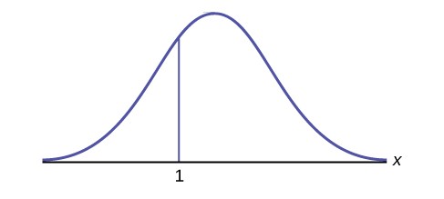
Figure 6.13

• What is the area to the right of one?

Figure 6.14

• Is P(x < 1) equal to P(x ≤ 1)? Why?

This OpenStax book is available for free at http://cnx.org/content/col11776/1.33

• How would you represent the area to the left of three in a probability statement?

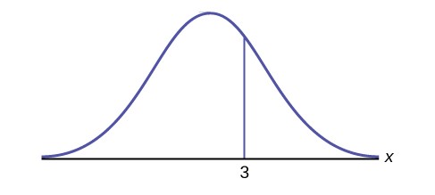
Figure 6.15

• What is the area to the right of three?

Figure 6.16

• If the area to the left of x in a normal distribution is 0.123, what is the area to the right of x?
• If the area to the right of x in a normal distribution is 0.543, what is the area to the left of x? Use the following information to answer the next four exercises:

X ~ N(54, 8)

• Find the probability that x > 56.
• Find the probability that x < 30.

52. X ~ N(6, 2)

Find the probability that x is between three and nine.

53. X ~ N(–3, 4)

Find the probability that x is between one and four.

54. X ~ N(4, 5)

Find the maximum of x in the bottom quartile.

• Use the following information to answer the next three exercise: The life of Sunshine CD players is normally distributed with a mean of 4.1 years and a standard deviation of 1.3 years. A CD player is guaranteed for three years. We are interested in the length of time a CD player lasts. Find the probability that a CD player will break down during the guarantee period.
• Sketch the situation. Label and scale the axes. Shade the region corresponding to the probability.

Figure 6.17

• P(0 < x < ) = (Use zero for the minimum value of x.)
• Find the probability that a CD player will last between 2.8 and six years.
• Sketch the situation. Label and scale the axes. Shade the region corresponding to the probability.

Figure 6.18

b. P( < x < ) =

• An experiment with a probability of success given as 0.40 is repeated 100 times. Use the normal distribution to approximate the binomial distribution, and find the probability the experiment will have at least 45 successes.
• An experiment with a probability of success given as 0.30 is repeated 90 times. Use the normal distribution to approximate the binomial distribution, and find the probability the experiment will have at least 22 successes.
• An experiment with a probability of success given as 0.40 is repeated 100 times. Use the normal distribution to approximate the binomial distribution, and find the probability the experiment will have from 35 to 45 successes.
• An experiment with a probability of success given as 0.30 is repeated 90 times. Use the normal distribution to approximate the binomial distribution, and find the probability the experiment will have from 26 to 30 successes.
• An experiment with a probability of success given as 0.40 is repeated 100 times. Use the normal distribution to approximate the binomial distribution, and find the probability the experiment will have at most 34 successes.
• An experiment with a probability of success given as 0.30 is repeated 90 times. Use the normal distribution to approximate the binomial distribution, and find the probability the experiment will have at most 34 successes.
• A multiple choice test has a probability any question will be guesses correctly of 0.25. There are 100 questions, and a student guesses at all of them. Use the normal distribution to approximate the binomial distribution, and determine the probability at least 30, but no more than 32, questions will be guessed correctly.
• A multiple choice test has a probability any question will be guesses correctly of 0.25. There are 100 questions, and a student guesses at all of them. Use the normal distribution to approximate the binomial distribution, and determine the probability at least 24, but no more than 28, questions will be guessed correctly.

This OpenStax book is available for free at http://cnx.org/content/col11776/1.33

HOMEWORK

6.1 The Standard Normal Distribution

Use the following information to answer the next two exercises: The patient recovery time from a particular surgical procedure is normally distributed with a mean of 5.3 days and a standard deviation of 2.1 days.

• What is the median recovery time? a. 2.7

b. 5.3

c. 7.4

d. 2.1

• What is the z-score for a patient who takes ten days to recover? a. 1.5

b. 0.2

c. 2.2

d. 7.3

• The length of time to find it takes to find a parking space at 9 A.M. follows a normal distribution with a mean of five minutes and a standard deviation of two minutes. If the mean is significantly greater than the standard deviation, which of the following statements is true?
• The data cannot follow the uniform distribution.
• The data cannot follow the exponential distribution..
• The data cannot follow the normal distribution.
• I only
• II only
• III only
• I, II, and III
• The heights of the 430 National Basketball Association players were listed on team rosters at the start of the 2005–2006 season. The heights of basketball players have an approximate normal distribution with mean, µ = 79 inches and a standard deviation, σ = 3.89 inches. For each of the following heights, calculate the z-score and interpret it using complete sentences.

• 77 inches
• 85 inches
• If an NBA player reported his height had a z-score of 3.5, would you believe him? Explain your answer.
• The systolic blood pressure (given in millimeters) of males has an approximately normal distribution with mean µ = 125 and standard deviation σ = 14. Systolic blood pressure for males follows a normal distribution.
• Calculate the z-scores for the male systolic blood pressures 100 and 150 millimeters.
• If a male friend of yours said he thought his systolic blood pressure was 2.5 standard deviations below the mean, but that he believed his blood pressure was between 100 and 150 millimeters, what would you say to him?
• Kyle’s doctor told him that the z-score for his systolic blood pressure is 1.75. Which of the following is the best interpretation of this standardized score? The systolic blood pressure (given in millimeters) of males has an approximately normal distribution with mean µ = 125 and standard deviation σ = 14. If X = a systolic blood pressure score then X ~ N (125, 14).
• Which answer(s) is/are correct?
• Kyle’s systolic blood pressure is 175.
• Kyle’s systolic blood pressure is 1.75 times the average blood pressure of men his age.
• Kyle’s systolic blood pressure is 1.75 above the average systolic blood pressure of men his age.
• Kyles’s systolic blood pressure is 1.75 standard deviations above the average systolic blood pressure for men.
• Calculate Kyle’s blood pressure.

• Height and weight are two measurements used to track a child’s development. The World Health Organization measures child development by comparing the weights of children who are the same height and the same gender. In 2009, weights for all 80 cm girls in the reference population had a mean µ = 10.2 kg and standard deviation σ = 0.8 kg. Weights are normally distributed. X ~ N(10.2, 0.8). Calculate the z-scores that correspond to the following weights and interpret them.
• 11 kg
• 7.9 kg
• 12.2 kg
• In 2005, 1,475,623 students heading to college took the SAT. The distribution of scores in the math section of the SAT follows a normal distribution with mean µ = 520 and standard deviation σ = 115.
• Calculate the z-score for an SAT score of 720. Interpret it using a complete sentence.
• What math SAT score is 1.5 standard deviations above the mean? What can you say about this SAT score?
• For 2012, the SAT math test had a mean of 514 and standard deviation 117. The ACT math test is an alternate to the SAT and is approximately normally distributed with mean 21 and standard deviation 5.3. If one person took the SAT math test and scored 700 and a second person took the ACT math test and scored 30, who did better with respect to the test they took?

6.3 Estimating the Binomial with the Normal Distribution

Use the following information to answer the next two exercises: The patient recovery time from a particular surgical procedure is normally distributed with a mean of 5.3 days and a standard deviation of 2.1 days.

• What is the probability of spending more than two days in recovery? a. 0.0580

b. 0.8447

c. 0.0553

d. 0.9420

Use the following information to answer the next three exercises: The length of time it takes to find a parking space at 9

A.M. follows a normal distribution with a mean of five minutes and a standard deviation of two minutes.

• Based upon the given information and numerically justified, would you be surprised if it took less than one minute to find a parking space?
• Yes
• No
• Unable to determine
• Find the probability that it takes at least eight minutes to find a parking space. a. 0.0001

b. 0.9270

c. 0.1862

d. 0.0668

• Seventy percent of the time, it takes more than how many minutes to find a parking space? a. 1.24

b. 2.41

c. 3.95

d. 6.05

• According to a study done by De Anza students, the height for Asian adult males is normally distributed with an average of 66 inches and a standard deviation of 2.5 inches. Suppose one Asian adult male is randomly chosen. Let X = height of the individual.

a. X ~ ( ,)

• Find the probability that the person is between 65 and 69 inches. Include a sketch of the graph, and write a probability statement.
• Would you expect to meet many Asian adult males over 72 inches? Explain why or why not, and justify your answer numerically.
• The middle 40% of heights fall between what two values? Sketch the graph, and write the probability statement.

This OpenStax book is available for free at http://cnx.org/content/col11776/1.33

• IQ is normally distributed with a mean of 100 and a standard deviation of 15. Suppose one individual is randomly chosen. Let X = IQ of an individual.

a. X ~ ( ,)

• Find the probability that the person has an IQ greater than 120. Include a sketch of the graph, and write a probability statement.
• MENSA is an organization whose members have the top 2% of all IQs. Find the minimum IQ needed to qualify for the MENSA organization. Sketch the graph, and write the probability statement.
• The percent of fat calories that a person in America consumes each day is normally distributed with a mean of about 36 and a standard deviation of 10. Suppose that one individual is randomly chosen. Let X = percent of fat calories.

a. X ~ ( ,)

• Find the probability that the percent of fat calories a person consumes is more than 40. Graph the situation. Shade in the area to be determined.
• Find the maximum number for the lower quarter of percent of fat calories. Sketch the graph and write the probability statement.
• Suppose that the distance of fly balls hit to the outfield (in baseball) is normally distributed with a mean of 250 feet and a standard deviation of 50 feet.
• If X = distance in feet for a fly ball, then X ~ ( ,)
• If one fly ball is randomly chosen from this distribution, what is the probability that this ball traveled fewer than 220 feet? Sketch the graph. Scale the horizontal axis X. Shade the region corresponding to the probability. Find the probability.
• In China, four-year-olds average three hours a day unsupervised. Most of the unsupervised children live in rural areas, considered safe. Suppose that the standard deviation is 1.5 hours and the amount of time spent alone is normally distributed. We randomly select one Chinese four-year-old living in a rural area. We are interested in the amount of time the child spends alone per day.
• In words, define the random variable X. b. X ~ ( ,)
• Find the probability that the child spends less than one hour per day unsupervised. Sketch the graph, and write the probability statement.
• What percent of the children spend over ten hours per day unsupervised?
• Seventy percent of the children spend at least how long per day unsupervised?
• In the 1992 presidential election, Alaska’s 40 election districts averaged 1,956.8 votes per district for President Clinton. The standard deviation was 572.3. (There are only 40 election districts in Alaska.) The distribution of the votes per district for President Clinton was bell-shaped. Let X = number of votes for President Clinton for an election district.
• State the approximate distribution of X.
• Is 1,956.8 a population mean or a sample mean? How do you know?
• Find the probability that a randomly selected district had fewer than 1,600 votes for President Clinton. Sketch the graph and write the probability statement.
• Find the probability that a randomly selected district had between 1,800 and 2,000 votes for President Clinton.
• Find the third quartile for votes for President Clinton.
• Suppose that the duration of a particular type of criminal trial is known to be normally distributed with a mean of 21 days and a standard deviation of seven days.
• In words, define the random variable X. b. X ~ ( ,)
• If one of the trials is randomly chosen, find the probability that it lasted at least 24 days. Sketch the graph and write the probability statement.
• Sixty percent of all trials of this type are completed within how many days?
• Terri Vogel, an amateur motorcycle racer, averages 129.71 seconds per 2.5 mile lap (in a seven-lap race) with a standard deviation of 2.28 seconds. The distribution of her race times is normally distributed. We are interested in one of her randomly selected laps.
• In words, define the random variable X. b. X ~ ( ,)
• Find the percent of her laps that are completed in less than 130 seconds.
• The fastest 3% of her laps are under .
• The middle 80% of her laps are from seconds to seconds.

• Thuy Dau, Ngoc Bui, Sam Su, and Lan Voung conducted a survey as to how long customers at Lucky claimed to wait in the checkout line until their turn. Let X = time in line. Table 6.1 displays the ordered real data (in minutes):

Table 6.1

• Calculate the sample mean and the sample standard deviation.
• Construct a histogram.
• Draw a smooth curve through the midpoints of the tops of the bars.
• In words, describe the shape of your histogram and smooth curve.
• Let the sample mean approximate μ and the sample standard deviation approximate σ. The distribution of X can then be approximated by X ~ ( ,)
• Use the distribution in part e to calculate the probability that a person will wait fewer than 6.1 minutes.
• Determine the cumulative relative frequency for waiting less than 6.1 minutes.
• Why aren’t the answers to part f and part g exactly the same?
• Why are the answers to part f and part g as close as they are?
• If only ten customers has been surveyed rather than 50, do you think the answers to part f and part g would have been closer together or farther apart? Explain your conclusion.
• Suppose that Ricardo and Anita attend different colleges. Ricardo’s GPA is the same as the average GPA at his school. Anita’s GPA is 0.70 standard deviations above her school average. In complete sentences, explain why each of the following statements may be false.
• Ricardo’s actual GPA is lower than Anita’s actual GPA.
• Ricardo is not passing because his z-score is zero.
• Anita is in the 70th percentile of students at her college.
• An expert witness for a paternity lawsuit testifies that the length of a pregnancy is normally distributed with a mean of 280 days and a standard deviation of 13 days. An alleged father was out of the country from 240 to 306 days before the birth of the child, so the pregnancy would have been less than 240 days or more than 306 days long if he was the father. The birth was uncomplicated, and the child needed no medical intervention. What is the probability that he was NOT the father? What is the probability that he could be the father? Calculate the z-scores first, and then use those to calculate the probability.
• A NUMMI assembly line, which has been operating since 1984, has built an average of 6,000 cars and trucks a week. Generally, 10% of the cars were defective coming off the assembly line. Suppose we draw a random sample of n = 100 cars. Let X represent the number of defective cars in the sample. What can we say about X in regard to the 68-95-99.7 empirical rule (one standard deviation, two standard deviations and three standard deviations from the mean are being referred to)? Assume a normal distribution for the defective cars in the sample.
• We flip a coin 100 times (n = 100) and note that it only comes up heads 20% (p = 0.20) of the time. The mean and standard deviation for the number of times the coin lands on heads is µ = 20 and σ = 4 (verify the mean and standard deviation). Solve the following:
• There is about a 68% chance that the number of heads will be somewhere between and .
• There is about a chance that the number of heads will be somewhere between 12 and 28.
• There is about a chance that the number of heads will be somewhere between eight and 32.

This OpenStax book is available for free at http://cnx.org/content/col11776/1.33

• A $1 scratch off lotto ticket will be a winner one out of five times. Out of a shipment of n = 190 lotto tickets, find the probability for the lotto tickets that there are
• somewhere between 34 and 54 prizes.
• somewhere between 54 and 64 prizes.
• more than 64 prizes.
• Facebook provides a variety of statistics on its Web site that detail the growth and popularity of the site.

On average, 28 percent of 18 to 34 year olds check their Facebook profiles before getting out of bed in the morning. Suppose this percentage follows a normal distribution with a standard deviation of five percent.

• A hospital has 49 births in a year. It is considered equally likely that a birth be a boy as it is the birth be a girl.
• What is the mean?
• What is the standard deviation?
• Can this binomial distribution be approximated with a normal distribution?
• If so, use the normal distribution to find the probability that at least 23 of the 49 births were boys.
• Historically, a final exam in a course is passed with a probability of 0.9. The exam is given to a group of 70 students.
• What is the mean of the binomial distribution?
• What is the standard deviation?
• Can this binomial distribution be approximate with a normal distribution?
• If so, use the normal distribution to find the probability that at least 60 of the students pass the exam?
• A tree in an orchard has 200 oranges. Of the oranges, 40 are not ripe. Use the normal distribution to approximate the binomial distribution, and determine the probability a box containing 35 oranges has at most two oranges that are not ripe.
• In a large city one in ten fire hydrants are in need of repair. If a crew examines 100 fire hydrants in a week, what is the probability they will find nine of fewer fire hydrants that need repair? Use the normal distribution to approximate the binomial distribution.
• On an assembly line it is determined 85% of the assembled products have no defects. If one day 50 items are assembled, what is the probability at least 4 and no more than 8 are defective. Use the normal distribution to approximate the binomial distribution.

REFERENCES

The Standard Normal Distribution

“Blood Pressure of Males and Females.” StatCruch, 2013. Available online at http://www.statcrunch.com/5.0/ viewreport.php?reportid=11960 (accessed May 14, 2013).

“The Use of Epidemiological Tools in Conflict-affected populations: Open-access educational resources for policy-makers: Calculation of z-scores.” London School of Hygiene and Tropical Medicine, 2009. Available online at http://conflict.lshtm.ac.uk/page_125.htm (accessed May 14, 2013).

“2012 College-Bound Seniors Total Group Profile Report.” CollegeBoard, 2012. Available online at http://media.collegeboard.com/digitalServices/pdf/research/TotalGroup-2012.pdf (accessed May 14, 2013).

“Digest of Education Statistics: ACT score average and standard deviations by sex and race/ethnicity and percentage of ACT test takers, by selected composite score ranges and planned fields of study: Selected years, 1995 through 2009.” National Center for Education Statistics. Available online at http://nces.ed.gov/programs/digest/d09/tables/dt09_147.asp (accessed May 14, 2013).

Data from the San Jose Mercury News.

Data from The World Almanac and Book of Facts.

“List of stadiums by capacity.” Wikipedia. Available online at https://en.wikipedia.org/wiki/List_of_stadiums_by_capacity (accessed May 14, 2013).

Data from the National Basketball Association. Available online at www.nba.com (accessed May 14, 2013).

Using the Normal Distribution

“Naegele’s rule.” Wikipedia. Available online at http://en.wikipedia.org/wiki/Naegele’s_rule (accessed May 14, 2013).

“403: NUMMI.” Chicago Public Media & Ira Glass, 2013. Available online at http://www.thisamericanlife.org/radio- archives/episode/403/nummi (accessed May 14, 2013).

“Scratch-OffLotteryTicketPlayingTips.”WinAtTheLottery.com,2013.Availableonlineat http://www.winatthelottery.com/public/department40.cfm (accessed May 14, 2013).

“Smart Phone Users, By The Numbers.” Visual.ly, 2013. Available online at http://visual.ly/smart-phone-users-numbers (accessed May 14, 2013).

“Facebook Statistics.” Statistics Brain. Available online at http://www.statisticbrain.com/facebook-statistics/(accessed May 14, 2013).

SOLUTIONS

1 ounces of water in a bottle

3 2

5 –4

7 –2

9 The mean becomes zero.

11 z = 2

13 z = 2.78

15 x = 20

17 x = 6.5

19 x = 1

21 x = 1.97

23 z = –1.67

25 z ≈ –0.33

27 0.67, right

29 3.14, left

31 about 68%

33 about 4%

35 between –5 and –1

37 about 50%

39 about 27%

41 The lifetime of a Sunshine CD player measured in years.

43 P(x < 1)

45 Yes, because they are the same in a continuous distribution: P(x = 1) = 0

47 1 – P(x < 3) or P(x > 3)

49 1 – 0.543 = 0.457

51 0.0013

53 0.1186

This OpenStax book is available for free at http://cnx.org/content/col11776/1.33

55

• Check student’s solution. b. 3, 0.1979

57 0.154

58 0.874

59 0.693

60 0.346

61 0.110

62 0.946

63 0.071

64 0.347

66 c

68

• Use the z-score formula. z = –0.5141. The height of 77 inches is 0.5141 standard deviations below the mean. An NBA player whose height is 77 inches is shorter than average.
• Use the z-score formula. z = 1.5424. The height 85 inches is 1.5424 standard deviations above the mean. An NBA player whose height is 85 inches is taller than average.
• Height = 79 + 3.5(3.89) = 92.615 inches, which is taller than 7 feet, 8 inches. There are very few NBA players this tall so the answer is no, not likely.

70

• iv
• Kyle’s blood pressure is equal to 125 + (1.75)(14) = 149.5.

72 Let X = an SAT math score and Y = an ACT math score.

a. X = 720 720 – 520

15

= 1.74 The exam score of 720 is 1.74 standard deviations above the mean of 520.

b. z = 1.5

The math SAT score is 520 + 1.5(115) ≈ 692.5. The exam score of 692.5 is 1.5 standard deviations above the mean of 520.

• X – µ = 700 – 514 ≈ 1.59, the z-score for the SAT. Y – µ = 30 – 21 ≈ 1.70, the z-scores for the ACT. With respect

σ117σ5.3

to the test they took, the person who took the ACT did better (has the higher z-score).

75 d

77

a. X ~ N(66, 2.5) b. 0.5404

c. No, the probability that an Asian male is over 72 inches tall is 0.0082

79

a. X ~ N(36, 10)

• The probability that a person consumes more than 40% of their calories as fat is 0.3446.
• Approximately 25% of people consume less than 29.26% of their calories as fat.

81

a. X = number of hours that a Chinese four-year-old in a rural area is unsupervised during the day. b. X ~ N(3, 1.5)

• The probability that the child spends less than one hour a day unsupervised is 0.0918.
• The probability that a child spends over ten hours a day unsupervised is less than 0.0001.
• 2.21 hours

83

a. X = the distribution of the number of days a particular type of criminal trial will take b. X ~ N(21, 7)

c. The probability that a randomly selected trial will last more than 24 days is 0.3336. d. 22.77

85

a. mean = 5.51, s = 2.15

• Check student’s solution.
• Check student’s solution.
• Check student’s solution. e. X ~ N(5.51, 2.15)

f. 0.6029

• The cumulative frequency for less than 6.1 minutes is 0.64.
• The answers to part f and part g are not exactly the same, because the normal distribution is only an approximation to the real one.
• The answers to part f and part g are close, because a normal distribution is an excellent approximation when the sample size is greater than 30.
• The approximation would have been less accurate, because the smaller sample size means that the data does not fit normal curve as well.

88

n = 100; p = 0.1; q = 0.9

μ = np = (100)(0.10) = 10

σ = npq = (100)(0.1)(0.9) = 3

i.z = ± 1 : x1 = µ + zσ = 10 + 1(3) = 13 and x2 = µ – zσ = 10 – 1(3) = 7.68% of the defective cars will fall between seven and 13.

ii.z = ± 2 : x1 = µ + zσ = 10 + 2(3) = 16 and x2 = µ – zσ = 10 – 2(3) = 4. 95 % of the defective cars will fall between four and 16

iii.z = ± 3 : x1 = µ + zσ = 10 + 3(3) = 19 and x2 = µ – zσ = 10 – 3(3) = 1. 99.7% of the defective cars will fall between one and 19.

90

n = 190; p = 1

5

= 0.2; q = 0.8

μ = np = (190)(0.2) = 38

(190)(0.2)(0.8)
σ = npq =

= 5.5136

• For this problem: P(34 < x < 54) = 0.7641
• For this problem: P(54 < x < 64) = 0.0018
• For this problem: P(x > 64) = 0.0000012 (approximately 0)

92

a. 24.5

This OpenStax book is available for free at http://cnx.org/content/col11776/1.33

b. 3.5

c. Yes

d. 0.67

93

a. 63

b. 2.5

c. Yes

d. 0.88

94 0.02

95 0.37

96 0.50

This OpenStax book is available for free at http://cnx.org/content/col11776/1.33