11 11 | THE CHI-SQUARE DISTRIBUTION

Figure 11.1 The chi-square distribution can be used to find relationships between two things, like grocery prices at different stores. (credit: Pete/flickr)

 

Introduction

 

Have you ever wondered if lottery winning numbers were evenly distributed or if some numbers occurred with a greater frequency? How about if the types of movies people preferred were different across different age groups? What about if a coffee machine was dispensing approximately the same amount of coffee each time? You could answer these questions by conducting a hypothesis test.

You will now study a new distribution, one that is used to determine the answers to such questions. This distribution is called the chi-square distribution.

In this chapter, you will learn the three major applications of the chi-square distribution:

• the goodness-of-fit test, which determines if data fit a particular distribution, such as in the lottery example
• the test of independence, which determines if events are independent, such as in the movie example
• the test of a single variance, which tests variability, such as in the coffee example

 

 

 

| Facts About the Chi-Square Distribution

The notation for the chi-square distribution is:

d f
χ ∼ χ 2

 

where df = degrees of freedom which depends on how chi-square is being used. (If you want to practice calculating chi- square probabilities then use df = n – 1. The degrees of freedom for the three major uses are each calculated differently.)

For the χ2 distribution, the population mean is μ = df and the population standard deviation is σ = 2(d f ) . The random variable is shown as χ2.

The random variable for a chi-square distribution with k degrees of freedom is the sum of k independent, squared standard normal variables.

χ2 = (Z1)2 + (Z2)2 + … + (Zk)2

• The curve is nonsymmetrical and skewed to the right.
• There is a different chi-square curve for each df.

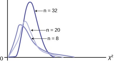
Figure 11.2

 

• The test statistic for any test is always greater than or equal to zero.
• 1,000
  When df > 90, the chi-square curve approximates the normal distribution. For X ~ χ 2the mean, μ = df = 1,000

2(1,000)
and the standard deviation, σ == 44.7. Therefore, X ~ N(1,000, 44.7), approximately.

• The mean, μ, is located just to the right of the peak.

 

| Test of a Single Variance

Thus far our interest has been exclusively on the population parameter μ or it’s counterpart in the binomial, p. Surely the mean of a population is the most critical piece of information to have, but in some cases we are interested in the variability of the outcomes of some distribution. In almost all production processes quality is measured not only by how closely the machine matches the target, but also the variability of the process. If one were filling bags with potato chips not only would there be interest in the average weight of the bag, but also how much variation there was in the weights. No one wants to be assured that the average weight is accurate when their bag has no chips. Electricity voltage may meet some average level, but great variability, spikes, can cause serious damage to electrical machines, especially computers. I would not only like to have a high mean grade in my classes, but also low variation about this mean. In short, statistical tests concerning the variance of a distribution have great value and many applications.

A test of a single variance assumes that the underlying distribution is normal. The null and alternative hypotheses are stated in terms of the population variance. The test statistic is:

⎛n – 1⎞s2

σ
2
χc2 = ⎝⎠

0

 

 

This OpenStax book is available for free at http://cnx.org/content/col11776/1.33

 

 

 

where:

• n = the total number of observations in the sample data
• s2 = sample variance
• 0
  σ 2 = hypothesized value of the population variance

0
•H0 : σ 2 = σ 2

0
•Ha : σ 2 ≠ σ 2

You may think of s as the random variable in this test. The number of degrees of freedom is df = n – 1. A test of a single variance may be right-tailed, left-tailed, or two-tailed. Example 11.1 will show you how to set up the null and alternative hypotheses. The null and alternative hypotheses contain statements about the population variance.

Example 11.1Math instructors are not only interested in how their students do on exams, on average, but how the exam scores vary. To many instructors, the variance (or standard deviation) may be more important than the average.Suppose a math instructor believes that the standard deviation for his final exam is five points. One of his best students thinks otherwise. The student claims that the standard deviation is more than five points. If the student were to conduct a hypothesis test, what would the null and alternative hypotheses be?Solution 11.1Even though we are given the population standard deviation, we can set up the test using the population variance as follows.• H0: σ2 ≤ 52• Ha: σ2 > 52
11.1 A SCUBA instructor wants to record the collective depths each of his students’ dives during their checkout. He is interested in how the depths vary, even though everyone should have been at the same depth. He believes the standard deviation is three feet. His assistant thinks the standard deviation is less than three feet. If the instructor were to conduct a test, what would the null and alternative hypotheses be?
Example 11.2With individual lines at its various windows, a post office finds that the standard deviation for waiting times for customers on Friday afternoon is 7.2 minutes. The post office experiments with a single, main waiting line and finds that for a random sample of 25 customers, the waiting times for customers have a standard deviation of 3.5 minutes on a Friday afternoon.With a significance level of 5%, test the claim that a single line causes lower variation among waiting times for customers.Solution 11.2Since the claim is that a single line causes less variation, this is a test of a single variance. The parameter is the population variance, σ2.Random Variable: The sample standard deviation, s, is the random variable. Let s = standard deviation for the

 

 

 

 

 

 

waiting times.

• H0: σ2 ≥ 7.22

• Ha: σ2 < 7.22

The word “less” tells you this is a left-tailed test.

24
Distribution for the test: χ 2 , where:

• n = the number of customers sampled

• df = n – 1 = 25 – 1 = 24

Calculate the test statistic:

χc2 = (n − 1)s2 = (25 − 1)(3.5)2 = 5.67

σ 27.22

where n = 25, s = 3.5, and σ = 7.2.

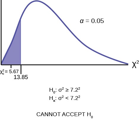
Figure 11.3

 

The graph of the Chi-square shows the distribution and marks the critical value with 24 degrees of freedom at 95% level of confidence, α = 0.05, 13.85. The critical value of 13.85 came from the Chi squared table which is read very much like the students t table. The difference is that the students t distribution is symmetrical and the Chi squared distribution is not. At the top of the Chi squared table we see not only the familiar 0.05, 0.10, etc. but also 0.95, 0.975, etc. These are the columns used to find the left hand critical value. The graph also marks the calculated χ2 test statistic of 5.67. Comparing the test statistic with the critical value, as we have done with all other hypothesis tests, we reach the conclusion.

Make a decision: Because the calculated test statistic is in the tail we cannot accept H0. This means that you reject σ2 ≥ 7.22. In other words, you do not think the variation in waiting times is 7.2 minutes or more; you think the variation in waiting times is less.

Conclusion: At a 5% level of significance, from the data, there is sufficient evidence to conclude that a single line causes a lower variation among the waiting times or with a single line, the customer waiting times vary less than 7.2 minutes.

 

 

 

This OpenStax book is available for free at http://cnx.org/content/col11776/1.33

 

 

 

Example 11.3

 

Professor Hadley has a weakness for cream filled donuts, but he believes that some bakeries are not properly filling the donuts. A sample of 24 donuts reveals a mean amount of filling equal to 0.04 cups, and the sample standard deviation is 0.11 cups. Professor Hadley has an interest in the average quantity of filling, of course, but he is particularly distressed if one donut is radically different from another. Professor Hadley does not like surprises.

Test at 95% the null hypothesis that the population variance of donut filling is significantly different from the average amount of filling.

 

Solution 11.3

This is clearly a problem dealing with variances. In this case we are testing a single sample rather than comparing two samples from different populations. The null and alternative hypotheses are thus:

H0 : σ 2 = 0.04

H0 : σ 2 ≠ 0.04

The test is set up as a two-tailed test because Professor Hadley has shown concern with too much variation in filling as well as too little: his dislike of a surprise is any level of filling outside the expected average of 0.04 cups. The test statistic is calculated to be:

⎛⎞ 2⎛⎞2

 

χc2 = ⎝n − 1⎠s

σo2

= ⎝24 − 1⎠0.11

0.042

= 6.9575

 

The calculated χ 2 test statistic, 6.96, is in the tail therefore at a 0.05 level of significance, we cannot accept the null hypothesis that the variance in the donut filling is equal to 0.04 cups. It seems that Professor Hadley is destined to meet disappointment with each bit.

 

 

 

 

 

 

 

 

 

 

 

 

 

 

Figure 11.4

 

 

11.3 The FCC conducts broadband speed tests to measure how much data per second passes between a consumer’s computer and the internet. As of August of 2012, the standard deviation of Internet speeds across Internet Service Providers (ISPs) was 12.2 percent. Suppose a sample of 15 ISPs is taken, and the standard deviation is 13.2. An analyst claims that the standard deviation of speeds is more than what was reported. State the null and alternative hypotheses, compute the degrees of freedom, the test statistic, sketch the graph of the distribution and mark the area associated with the level of confidence, and draw a conclusion. Test at the 1% significance level.

 

 

 

| Goodness-of-Fit Test

In this type of hypothesis test, you determine whether the data “fit” a particular distribution or not. For example, you may suspect your unknown data fit a binomial distribution. You use a chi-square test (meaning the distribution for the hypothesis test is chi-square) to determine if there is a fit or not. The null and the alternative hypotheses for this test may be written in sentences or may be stated as equations or inequalities.

The test statistic for a goodness-of-fit test is:

Σ (O − E)2

kE

where:

• O = observed values (data)
• E = expected values (from theory)
• k = the number of different data cells or categories

E
The observed values are the data values and the expected values are the values you would expect to get if the null hypothesis were true. There are n terms of the form (O − E)2 .

The number of degrees of freedom is df = (number of categories – 1).

NOTEThe number of expected values inside each cell needs to be at least five in order to use this test.
Example 11.4Absenteeism of college students from math classes is a major concern to math instructors because missing class appears to increase the drop rate. Suppose that a study was done to determine if the actual student absenteeism rate follows faculty perception. The faculty expected that a group of 100 students would miss class according to Table 11.1.Table 11.1A random survey across all mathematics courses was then done to determine the actual number (observed) of absences in a course. The chart in Table 11.2 displays the results of that survey.
The goodness-of-fit test is almost always right-tailed. If the observed values and the corresponding expected values are not close to each other, then the test statistic can get very large and will be way out in the right tail of the chi-square curve.

 

 

 

 

 

 

 

 

 

 

 

 

 

 

 

 

 

 

 

 

 

 

 

This OpenStax book is available for free at http://cnx.org/content/col11776/1.33

 

 

 

 

Table 11.2

 

 

 

Determine the null and alternative hypotheses needed to conduct a goodness-of-fit test.

H0: Student absenteeism fits faculty perception.

 

The alternative hypothesis is the opposite of the null hypothesis.

Ha: Student absenteeism does not fit faculty perception.

a. Can you use the information as it appears in the charts to conduct the goodness-of-fit test?

 

Solution 11.4

• No. Notice that the expected number of absences for the “12+” entry is less than five (it is two). Combine that group with the “9–11” group to create new tables where the number of students for each entry are at least five. The new results are in Table 11.2 and Table 11.3.

 

Table 11.3

 

 

Table 11.4

 

 

• What is the number of degrees of freedom (df)?

 

Solution 11.4

• There are four “cells” or categories in each of the new tables.

df = number of cells – 1 = 4 – 1 = 3

 

11.4 A factory manager needs to understand how many products are defective versus how many are produced. The number of expected defects is listed in Table 11.5.Table 11.5A random sample was taken to determine the actual number of defects. Table 11.6 shows the results of the survey.Table 11.6State the null and alternative hypotheses needed to conduct a goodness-of-fit test, and state the degrees of freedom.

 

 

 

 

 

 

 

 

 

 

 

 

 

 

 

 

 

 

 

 

 

 

 

 

 

 

 

 

 

 

 

 

 

 

 

 

 

 

 

 

 

Example 11.5Employers want to know which days of the week employees are absent in a five-day work week. Most employers would like to believe that employees are absent equally during the week. Suppose a random sample of 60 managers were asked on which day of the week they had the highest number of employee absences. The results were distributed as in Table 11.6. For the population of employees, do the days for the highest number of absences occur with equal frequencies during a five-day work week? Test at a 5% significance level.Table 11.7 Day of the Week Employees were Most AbsentSolution 11.5The null and alternative hypotheses are:H0: The absent days occur with equal frequencies, that is, they fit a uniform distribution.
This OpenStax book is available for free at http://cnx.org/content/col11776/1.33

 

 

 

 

• Ha: The absent days occur with unequal frequencies, that is, they do not fit a uniform distribution.

If the absent days occur with equal frequencies, then, out of 60 absent days (the total in the sample: 15 + 12 + 9

+ 9 + 15 = 60), there would be 12 absences on Monday, 12 on Tuesday, 12 on Wednesday, 12 on Thursday, and 12 on Friday. These numbers are the expected (E) values. The values in the table are the observed (O) values or data.

This time, calculate the χ2 test statistic by hand. Make a chart with the following headings and fill in the columns:

• Expected (E) values (12, 12, 12, 12, 12)

• Observed (O) values (15, 12, 9, 9, 15)

• (O – E)

• (O – E)2

•
(O – E)2 E

Now add (sum) the last column. The sum is three. This is the χ2 test statistic.

The calculated test statistics is 3 and the critical value of the χ2 distribution at 4 degrees of freedom the 0.05 level of confidence is 9.48. This value is found in the χ2 table at the 0.05 column on the degrees of freedom row 4.

The degrees of freedom are the number of cells – 1 = 5 – 1 = 4

Next, complete a graph like the following one with the proper labeling and shading. (You should shade the right tail.)

 

 

 

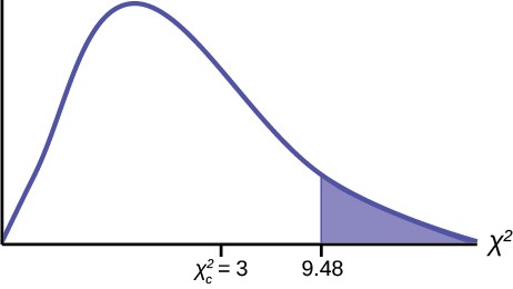
Figure 11.5

χc2 = Σ (O − E)2 = 3

 

 

kE

The decision is not to reject the null hypothesis because the calculated value of the test statistic is not in the tail of the distribution.

Conclusion: At a 5% level of significance, from the sample data, there is not sufficient evidence to conclude that the absent days do not occur with equal frequencies.

 

11.5 Teachers want to know which night each week their students are doing most of their homework. Most teachers think that students do homework equally throughout the week. Suppose a random sample of 56 students were asked on

 

which night of the week they did the most homework. The results were distributed as in Table 11.8.Table 11.8From the population of students, do the nights for the highest number of students doing the majority of their homework occur with equal frequencies during a week? What type of hypothesis test should you use?

 

 

 

 

 

 

 

 

 

 

 

 

 

 

 

 

 

 

 

 

 

 

 

 

 

 

 

 

 

 

 

 

 

 

 

 

 

Example 11.6One study indicates that the number of televisions that American families have is distributed (this is the givendistribution for the American population) as in Table 11.9.Table 11.9The table contains expected (E) percents.A random sample of 600 families in the far western United States resulted in the data in Table 11.10.Table 11.10The table contains observed (O) frequency values.At the 1% significance level, does it appear that the distribution “number of televisions” of far western United States families is different from the distribution for the American population as a whole?
This OpenStax book is available for free at http://cnx.org/content/col11776/1.33

 

 

 

 

Solution 11.6

This problem asks you to test whether the far western United States families distribution fits the distribution of the American families. This test is always right-tailed.

The first table contains expected percentages. To get expected (E) frequencies, multiply the percentage by 600. The expected frequencies are shown in Table 11.10.

 

Table 11.11

 

 

Therefore, the expected frequencies are 60, 96, 330, 66, and 48.

H0: The “number of televisions” distribution of far western United States families is the same as the “number of televisions” distribution of the American population.

Ha: The “number of televisions” distribution of far western United States families is different from the “number of televisions” distribution of the American population.

4
Distribution for the test: χ 2 where df = (the number of cells) – 1 = 5 – 1 = 4.

Calculate the test statistic: χ2 = 29.65

Graph:

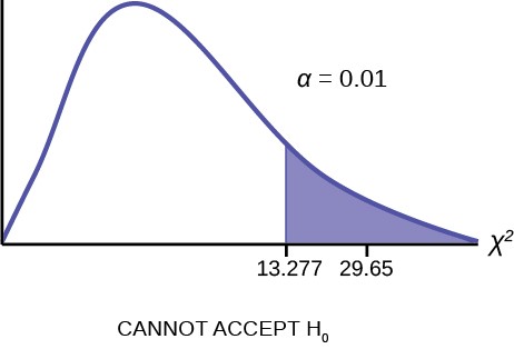
Figure 11.6

 

The graph of the Chi-square shows the distribution and marks the critical value with four degrees of freedom at 99% level of confidence, α = .01, 13.277. The graph also marks the calculated chi squared test statistic of 29.65. Comparing the test statistic with the critical value, as we have done with all other hypothesis tests, we reach the conclusion.

 

 

 

 

 

Make a decision: Because the test statistic is in the tail of the distribution we cannot accept the null hypothesis.

This means you reject the belief that the distribution for the far western states is the same as that of the American population as a whole.

11.6 The expected percentage of the number of pets students have in their homes is distributed (this is the given distribution for the student population of the United States) as in Table 11.12.Table 11.12A random sample of 1,000 students from the Eastern United States resulted in the data in Table 11.13.Table 11.13At the 1% significance level, does it appear that the distribution “number of pets” of students in the Eastern United States is different from the distribution for the United States student population as a whole?
Conclusion: At the 1% significance level, from the data, there is sufficient evidence to conclude that the “number of televisions” distribution for the far western United States is different from the “number of televisions” distribution for the American population as a whole.

 

 

 

 

 

 

 

 

 

 

 

 

 

 

 

 

 

 

 

 

 

Example 11.7Suppose you flip two coins 100 times. The results are 20 HH, 27 HT, 30 TH, and 23 TT. Are the coins fair? Test at a 5% significance level.Solution 11.7This problem can be set up as a goodness-of-fit problem. The sample space for flipping two fair coins is {HH, HT,

 

 

This OpenStax book is available for free at http://cnx.org/content/col11776/1.33

 

 

 

 

 

TH, TT}. Out of 100 flips, you would expect 25 HH, 25 HT, 25 TH, and 25 TT. This is the expected distribution from the binomial probability distribution. The question, “Are the coins fair?” is the same as saying, “Does the distribution of the coins (20 HH, 27 HT, 30 TH, 23 TT) fit the expected distribution?”

Random Variable: Let X = the number of heads in one flip of the two coins. X takes on the values 0, 1, 2. (There are 0, 1, or 2 heads in the flip of two coins.) Therefore, the number of cells is three. Since X = the number of heads, the observed frequencies are 20 (for two heads), 57 (for one head), and 23 (for zero heads or both tails). The expected frequencies are 25 (for two heads), 50 (for one head), and 25 (for zero heads or both tails). This test is right-tailed.

H0: The coins are fair.

Ha: The coins are not fair.

2
Distribution for the test: χ 2 where df = 3 – 1 = 2.

Calculate the test statistic: χ2 = 2.14

Graph:

Figure 11.7

 

The graph of the Chi-square shows the distribution and marks the critical value with two degrees of freedom at 95% level of confidence, α = 0.05, 5.991. The graph also marks the calculated χ2 test statistic of 2.14. Comparing the test statistic with the critical value, as we have done with all other hypothesis tests, we reach the conclusion.

Conclusion: There is insufficient evidence to conclude that the coins are not fair: we cannot reject the null hypothesis that the coins are fair.

 

 

| Test of Independence

⋅
Tests of independence involve using a contingency table of observed (data) values. The test statistic for a test of independence is similar to that of a goodness-of-fit test:

 

 

 

 

where:

• O = observed values

(iΣj)

(O – E)2 E

 

 

• E = expected values
• i = the number of rows in the table
• E
  j = the number of columns in the table There are i ⋅ j terms of the form (O – E)2 .

NOTEThe expected value inside each cell needs to be at least five in order for you to use this test.
A test of independence determines whether two factors are independent or not. You first encountered the term independence in Section 3.2 earlier. As a review, consider the following example.

 

Example 11.8

 

Suppose A = a speeding violation in the last year and B = a cell phone user while driving. If A and B are independent then P(A ∩ B) = P(A)P(B). A ∩ B is the event that a driver received a speeding violation last year and also used a cell phone while driving. Suppose, in a study of drivers who received speeding violations

in the last year, and who used cell phone while driving, that 755 people were surveyed. Out of the 755, 70 had a speeding violation and 685 did not; 305 used cell phones while driving and 450 did not.

Let y = expected number of drivers who used a cell phone while driving and received speeding violations. If A and B are independent, then P(A ∩ B) = P(A)P(B). By substitution,

y = ⎛ 70 ⎞⎛305⎞

755⎝755⎠⎝755⎠

755
Solve for y: y = (70)(305) = 28.3

About 28 people from the sample are expected to use cell phones while driving and to receive speeding violations.

In a test of independence, we state the null and alternative hypotheses in words. Since the contingency table consists of two factors, the null hypothesis states that the factors are independent and the alternative hypothesis states that they are not independent (dependent). If we do a test of independence using the example, then the null hypothesis is:

H0 : Being a cell phone user while driving and receiving a speeding violation are independent events; in other words, they have no effect on each other.

If the null hypothesis were true, we would expect about 28 people to use cell phones while driving and to receive a speeding violation.

The test of independence is always right-tailed because of the calculation of the test statistic. If the expected and observed values are not close together, then the test statistic is very large and way out in the right tail of the chi-square curve, as it is in a goodness-of-fit.

The number of degrees of freedom for the test of independence is:

df = (number of columns – 1)(number of rows – 1)

The following formula calculates the expected number (E):

E =
(row total)(column total) total number surveyed

 

 

 

 

 

 

 

This OpenStax book is available for free at http://cnx.org/content/col11776/1.33

 

 

 

11.8 A sample of 300 students is taken. Of the students surveyed, 50 were music students, while 250 were not. Ninety- seven of the 300 surveyed were on the honor roll, while 203 were not. If we assume being a music student and being on the honor roll are independent events, what is the expected number of music students who are also on the honor roll?

 

Example 11.9

 

A volunteer group, provides from one to nine hours each week with disabled senior citizens. The program recruits among community college students, four-year college students, and nonstudents. In Table 11.14 is a sample of the adult volunteers and the number of hours they volunteer per week.

 

Table 11.14 Number of Hours Worked Per Week by Volunteer Type (Observed) The table contains observed (O) values (data).

 

 

Is the number of hours volunteered independent of the type of volunteer?

 

Solution 11.9

The observed table and the question at the end of the problem, “Is the number of hours volunteered independent of the type of volunteer?” tell you this is a test of independence. The two factors are number of hours volunteered and type of volunteer. This test is always right-tailed.

H0: The number of hours volunteered is independent of the type of volunteer. Ha: The number of hours volunteered is dependent on the type of volunteer. The expected result are in Table 11.14.

 

Table 11.15 Number of Hours Worked Per Week by Volunteer Type (Expected) The table contains expected (E) values (data).

 

 

For example, the calculation for the expected frequency for the top left cell is

E = (row total)(column total) = (255)(298) = 90.57

total number surveyed839

Calculate the test statistic: χ2 = 12.99 (calculator or computer)

 

 

 

4
Distribution for the test: χ 2

df = (3 columns – 1)(3 rows – 1) = (2)(2) = 4

Graph:

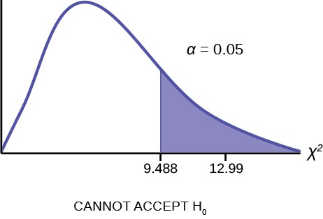
Figure 11.8

 

The graph of the Chi-square shows the distribution and marks the critical value with four degrees of freedom at 95% level of confidence, α = 0.05, 9.488. The graph also marks the calculated χc2 test statistic of 12.99. Comparing the test statistic with the critical value, as we have done with all other hypothesis tests, we reach the conclusion.

Make a decision: Because the calculated test statistic is in the tail we cannot accept H0. This means that the factors are not independent.

Conclusion: At a 5% level of significance, from the data, there is sufficient evidence to conclude that the number of hours volunteered and the type of volunteer are dependent on one another.

For the example in Table 11.14, if there had been another type of volunteer, teenagers, what would the degrees of freedom be?

 

 

 

 

 

 

 

 

 

 

 

 

 

 

 

 

 

 

 

 

 

This OpenStax book is available for free at http://cnx.org/content/col11776/1.33

 

11.9 The Bureau of Labor Statistics gathers data about employment in the United States. A sample is taken to calculate the number of U.S. citizens working in one of several industry sectors over time. Table 11.16 shows the results:Table 11.16We want to know if the change in the number of jobs is independent of the change in years. State the null and alternative hypotheses and the degrees of freedom.
Example 11.10De Anza College is interested in the relationship between anxiety level and the need to succeed in school. A random sample of 400 students took a test that measured anxiety level and need to succeed in school. Table11.17 shows the results. De Anza College wants to know if anxiety level and need to succeed in school are independent events.Table 11.17 Need to Succeed in School vs. Anxiety Levela. How many high anxiety level students are expected to have a high need to succeed in school?Solution 11.10a. The column total for a high anxiety level is 57. The row total for high need to succeed in school is 155. The sample size or total surveyed is 400.

 

 

 

 

 

 

 

 

 

 

 

 

 

 

 

 

 

 

 

 

 

 

 

 

 

 

 

 

 

E = (row total)(column total) = 155 ⋅ 57 = 22.09

total surveyed400

The expected number of students who have a high anxiety level and a high need to succeed in school is about 22.

 

b. If the two variables are independent, how many students do you expect to have a low need to succeed in school and a med-low level of anxiety?

 

Solution 11.10

b. The column total for a med-low anxiety level is 63. The row total for a low need to succeed in school is 52. The sample size or total surveyed is 400.

c. E =
(row total)(column total) =

total surveyed

 

Solution 11.10

c. E == 8.19
(row total)(column total) total surveyed

d. The expected number of students who have a med-low anxiety level and a low need to succeed in school is about .

 

Solution 11.10

d. 8

 

 

| Test for Homogeneity

NOTEThe expected value inside each cell needs to be at least five in order for you to use this test.
The goodness–of–fit test can be used to decide whether a population fits a given distribution, but it will not suffice to decide whether two populations follow the same unknown distribution. A different test, called the test for homogeneity, can be used to draw a conclusion about whether two populations have the same distribution. To calculate the test statistic for a test for homogeneity, follow the same procedure as with the test of independence.

 

Hypotheses

 

H0: The distributions of the two populations are the same.

Ha: The distributions of the two populations are not the same.

Test Statistic

Use a χ 2 test statistic. It is computed in the same way as the test for independence.

Degrees of Freedom (df) df = number of columns – 1 Requirements

All values in the table must be greater than or equal to five.

Common Uses

Comparing two populations. For example: men vs. women, before vs. after, east vs. west. The variable is categorical with more than two possible response values.

 

 

This OpenStax book is available for free at http://cnx.org/content/col11776/1.33

 

 

Example 11.11

 

Do male and female college students have the same distribution of living arrangements? Use a level of significance of 0.05. Suppose that 250 randomly selected male college students and 300 randomly selected female college students were asked about their living arrangements: dormitory, apartment, with parents, other. The results are shown in Table 11.17. Do male and female college students have the same distribution of living arrangements?

 

Table 11.18 Distribution of Living Arragements for College Males and College Females

 

 

 

Solution 11.11

H0: The distribution of living arrangements for male college students is the same as the distribution of living arrangements for female college students.

 

Ha: The distribution of living arrangements for male college students is not the same as the distribution of living arrangements for female college students.

 

Degrees of Freedom (df):

df = number of columns – 1 = 4 – 1 = 3

 

3
Distribution for the test: χ 2

 

Calculate the test statistic: χc2 = 10.129

 

 

 

 

 

 

 

 

 

 

 

 

 

 

 

 

 

 

 

Figure 11.9

 

 

The graph of the Chi-square shows the distribution and marks the critical value with three degrees of freedom

 

 

 

 

 

at 95% level of confidence, α = 0.05, 7.815. The graph also marks the calculated χ2 test statistic of 10.129. Comparing the test statistic with the critical value, as we have done with all other hypothesis tests, we reach the conclusion.

 

Make a decision: Because the calculated test statistic is in the tail we cannot accept H0. This means that the distributions are not the same.

 

Conclusion: At a 5% level of significance, from the data, there is sufficient evidence to conclude that the distributions of living arrangements for male and female college students are not the same.

 

11.11 Do families and singles have the same distribution of cars? Use a level of significance of 0.05. Suppose that 100 randomly selected families and 200 randomly selected singles were asked what type of car they drove: sport, sedan, hatchback, truck, van/SUV. The results are shown in Table 11.19. Do families and singles have the same distribution of cars? Test at a level of significance of 0.05.Table 11.19
Notice that the conclusion is only that the distributions are not the same. We cannot use the test for homogeneity to draw any conclusions about how they differ.

 

 

 

 

 

 

 

 

 

 

 

 

 

 

 

 

 

 

 

 

 

 

 

 

 

 

 

 

 

 

 

 

 

 

 

 

 

11.11 Ivy League schools receive many applications, but only some can be accepted. At the schools listed inTable 11.20, two types of applications are accepted: regular and early decision.Table 11.20We want to know if the number of regular applications accepted follows the same distribution as the number of early applications accepted. State the null and alternative hypotheses, the degrees of freedom and the test statistic, sketch the graph of the χ2 distribution and show the critical value and the calculated value of the test statistic, and draw a conclusion about the test of homogeneity.
This OpenStax book is available for free at http://cnx.org/content/col11776/1.33

 

 

 

| Comparison of the Chi-Square Tests

Above the χ2 test statistic was used in three different circumstances. The following bulleted list is a summary of which χ2

test is the appropriate one to use in different circumstances.

• Goodness-of-Fit: Use the goodness-of-fit test to decide whether a population with an unknown distribution “fits” a known distribution. In this case there will be a single qualitative survey question or a single outcome of an experiment from a single population. Goodness-of-Fit is typically used to see if the population is uniform (all outcomes occur with equal frequency), the population is normal, or the population is the same as another population with a known distribution. The null and alternative hypotheses are:

H0: The population fits the given distribution.

Ha: The population does not fit the given distribution.

• Independence: Use the test for independence to decide whether two variables (factors) are independent or dependent. In this case there will be two qualitative survey questions or experiments and a contingency table will be constructed. The goal is to see if the two variables are unrelated (independent) or related (dependent). The null and alternative hypotheses are:

H0: The two variables (factors) are independent.

Ha: The two variables (factors) are dependent.

• Homogeneity: Use the test for homogeneity to decide if two populations with unknown distributions have the same distribution as each other. In this case there will be a single qualitative survey question or experiment given to two different populations. The null and alternative hypotheses are:

H0: The two populations follow the same distribution.

Ha: The two populations have different distributions.

 

 

 

KEY TERMS

Contingency Table a table that displays sample values for two different factors that may be dependent or contingent on one another; it facilitates determining conditional probabilities.

 

Goodness-of-Fit a hypothesis test that compares expected and observed values in order to look for significant differences within one non-parametric variable. The degrees of freedom used equals the (number of categories – 1).

 

Test for Homogeneity a test used to draw a conclusion about whether two populations have the same distribution. The degrees of freedom used equals the (number of columns – 1).

 

Test of Independence a hypothesis test that compares expected and observed values for contingency tables in order to test for independence between two variables. The degrees of freedom used equals the (number of columns – 1) multiplied by the (number of rows – 1).

 

CHAPTER REVIEW

 

Facts About the Chi-Square Distribution

The chi-square distribution is a useful tool for assessment in a series of problem categories. These problem categories include primarily (i) whether a data set fits a particular distribution, (ii) whether the distributions of two populations are the same, (iii) whether two events might be independent, and (iv) whether there is a different variability than expected within a population.

An important parameter in a chi-square distribution is the degrees of freedom df in a given problem. The random variable in the chi-square distribution is the sum of squares of df standard normal variables, which must be independent. The key characteristics of the chi-square distribution also depend directly on the degrees of freedom.

The chi-square distribution curve is skewed to the right, and its shape depends on the degrees of freedom df. For df > 90, the curve approximates the normal distribution. Test statistics based on the chi-square distribution are always greater than or equal to zero. Such application tests are almost always right-tailed tests.

 

Test of a Single Variance

To test variability, use the chi-square test of a single variance. The test may be left-, right-, or two-tailed, and its hypotheses are always expressed in terms of the variance (or standard deviation).

 

Goodness-of-Fit Test

To assess whether a data set fits a specific distribution, you can apply the goodness-of-fit hypothesis test that uses the chi-square distribution. The null hypothesis for this test states that the data come from the assumed distribution. The test compares observed values against the values you would expect to have if your data followed the assumed distribution. The test is almost always right-tailed. Each observation or cell category must have an expected value of at least five.

 

Test of Independence

To assess whether two factors are independent or not, you can apply the test of independence that uses the chi-square distribution. The null hypothesis for this test states that the two factors are independent. The test compares observed values to expected values. The test is right-tailed. Each observation or cell category must have an expected value of at least 5.

 

Test for Homogeneity

To assess whether two data sets are derived from the same distribution—which need not be known, you can apply the test for homogeneity that uses the chi-square distribution. The null hypothesis for this test states that the populations of the two data sets come from the same distribution. The test compares the observed values against the expected values if the two populations followed the same distribution. The test is right-tailed. Each observation or cell category must have an expected value of at least five.

 

Comparison of the Chi-Square Tests

The goodness-of-fit test is typically used to determine if data fits a particular distribution. The test of independence makes use of a contingency table to determine the independence of two factors. The test for homogeneity determines whether two

 

 

 

 

This OpenStax book is available for free at http://cnx.org/content/col11776/1.33

 

 

 

populations come from the same distribution, even if this distribution is unknown.

 

 

 

FORMULA REVIEW

 

 

Facts About the Chi-Square Distribution

χ2 = (Z1)2 + (Z2)2 + … (Zdf)2 chi-square distribution random variable

μχ2 = df chi-square distribution population mean

2⎛d f ⎞⎝⎠
o χ 2 =Chi-Square distribution population standard deviation

 

Test of a Single Variance

2
χ 2 = (n − 1)s2 Test of a single variance statistic where:

σ

O: observed values

E: expected values

 

k: number of different data cells or categories

df = k − 1 degrees of freedom

 

Test of Independence

 

Test of Independence

• The number of degrees of freedom is equal to (number of columns – 1)(number of rows – 1).

(O − E)2

 

0

n: sample size

• 
  The test statistic is ∑

i ⋅ j

Ewhere O =

 

s: sample standard deviation

σ0 : hypothesized value of the population standard deviation

df = n – 1 Degrees of freedom

 

Test of a Single Variance

• Use the test to determine variation.
• The degrees of freedom is the number of samples – 1.

observed values, E = expected values, i = the number of rows in the table, and j = the number of columns in the table.

• If the null hypothesis is true, the expected number

E =.
(row total)(column total) total surveyed

 

• Test for Homogeneity

 

(n – 1)s2

∑ (O − E)2

Homogeneity test statistic where: O =

 

• σ
  The test statistic is

2, where n = sample size,

0

i ⋅ jE

 

s2 = sample variance, and σ2 = population variance.

• The test may be left-, right-, or two-tailed.

 

11.3 Goodness-of-Fit Test

observed values

E = expected values

i = number of rows in data contingency table

j = number of columns in data contingency table

df = (i −1)(j −1) Degrees of freedom

 

∑ (O − E)2

goodness-of-fit test statistic where:

 

kE

 

PRACTICE

 

Facts About the Chi-Square Distribution

• If the number of degrees of freedom for a chi-square distribution is 25, what is the population mean and standard deviation?
• If df > 90, the distribution is . If df = 15, the distribution is .
• When does the chi-square curve approximate a normal distribution?
• Where is μ located on a chi-square curve?

 

 

 

• Is it more likely the df is 90, 20, or two in the graph?

 

Figure 11.10

 

Test of a Single Variance

Use the following information to answer the next three exercises: An archer’s standard deviation for his hits is six (data is measured in distance from the center of the target). An observer claims the standard deviation is less.

• What type of test should be used?
• State the null and alternative hypotheses.
• Is this a right-tailed, left-tailed, or two-tailed test?

 

Use the following information to answer the next three exercises: The standard deviation of heights for students in a school is 0.81. A random sample of 50 students is taken, and the standard deviation of heights of the sample is 0.96. A researcher in charge of the study believes the standard deviation of heights for the school is greater than 0.81.

• What type of test should be used?
• State the null and alternative hypotheses.
• df =

 

Use the following information to answer the next four exercises: The average waiting time in a doctor’s office varies. The standard deviation of waiting times in a doctor’s office is 3.4 minutes. A random sample of 30 patients in the doctor’s office has a standard deviation of waiting times of 4.1 minutes. One doctor believes the variance of waiting times is greater than originally thought.

• What type of test should be used?
• What is the test statistic?
• What can you conclude at the 5% significance level?

 

Goodness-of-Fit Test

Determine the appropriate test to be used in the next three exercises.

• An archeologist is calculating the distribution of the frequency of the number of artifacts she finds in a dig site. Based on previous digs, the archeologist creates an expected distribution broken down by grid sections in the dig site. Once the site has been fully excavated, she compares the actual number of artifacts found in each grid section to see if her expectation was accurate.

 

 

 

 

 

 

This OpenStax book is available for free at http://cnx.org/content/col11776/1.33

 

 

 

• An economist is deriving a model to predict outcomes on the stock market. He creates a list of expected points on the stock market index for the next two weeks. At the close of each day’s trading, he records the actual points on the index. He wants to see how well his model matched what actually happened.
• A personal trainer is putting together a weight-lifting program for her clients. For a 90-day program, she expects each client to lift a specific maximum weight each week. As she goes along, she records the actual maximum weights her clients lifted. She wants to know how well her expectations met with what was observed.

Use the following information to answer the next five exercises: A teacher predicts that the distribution of grades on the final exam will be and they are recorded in Table 11.21.

 

Table 11.21

 

The actual distribution for a class of 20 is in Table 11.22.

 

Table 11.22

 

• d f =
• State the null and alternative hypotheses.
• χ2 test statistic =
• At the 5% significance level, what can you conclude?

 

Use the following information to answer the next nine exercises: The following data are real. The cumulative number of AIDS cases reported for Santa Clara County is broken down by ethnicity as in Table 11.23.

 

Table 11.23

 

The percentage of each ethnic group in Santa Clara County is as in Table 11.24.

 

 

 

Table 11.24

 

• If the ethnicities of AIDS victims followed the ethnicities of the total county population, fill in the expected number of cases per ethnic group.

Perform a goodness-of-fit test to determine whether the occurrence of AIDS cases follows the ethnicities of the general population of Santa Clara County.

23. H0:

• Ha:
• Is this a right-tailed, left-tailed, or two-tailed test?
• degrees of freedom =
• χ2 test statistic =
• Graph the situation. Label and scale the horizontal axis. Mark the mean and test statistic. Shade in the region corresponding to the confidence level.

 

Figure 11.11

Let α = 0.05

Decision:

Reason for the Decision:

Conclusion (write out in complete sentences):

• Does it appear that the pattern of AIDS cases in Santa Clara County corresponds to the distribution of ethnic groups in this county? Why or why not?

 

Test of Independence

Determine the appropriate test to be used in the next three exercises.

 

 

 

 

This OpenStax book is available for free at http://cnx.org/content/col11776/1.33

 

 

 

• A pharmaceutical company is interested in the relationship between age and presentation of symptoms for a common viral infection. A random sample is taken of 500 people with the infection across different age groups.
• The owner of a baseball team is interested in the relationship between player salaries and team winning percentage. He takes a random sample of 100 players from different organizations.
• A marathon runner is interested in the relationship between the brand of shoes runners wear and their run times. She takes a random sample of 50 runners and records their run times as well as the brand of shoes they were wearing.

 

Use the following information to answer the next seven exercises: Transit Railroads is interested in the relationship between travel distance and the ticket class purchased. A random sample of 200 passengers is taken. Table 11.25 shows the results. The railroad wants to know if a passenger’s choice in ticket class is independent of the distance they must travel.

 

Table 11.25

 

• State the hypotheses.

H0:

Ha:

• df =
• How many passengers are expected to travel between 201 and 300 miles and purchase second-class tickets?
• How many passengers are expected to travel between 401 and 500 miles and purchase first-class tickets?
• What is the test statistic?
• What can you conclude at the 5% level of significance?

 

Use the following information to answer the next eight exercises: An article in the New England Journal of Medicine, discussed a study on smokers in California and Hawaii. In one part of the report, the self-reported ethnicity and smoking levels per day were given. Of the people smoking at most ten cigarettes per day, there were 9,886 African Americans, 2,745 Native Hawaiians, 12,831 Latinos, 8,378 Japanese Americans and 7,650 whites. Of the people smoking 11 to 20 cigarettes per day, there were 6,514 African Americans, 3,062 Native Hawaiians, 4,932 Latinos, 10,680 Japanese Americans, and 9,877 whites. Of the people smoking 21 to 30 cigarettes per day, there were 1,671 African Americans, 1,419 Native Hawaiians, 1,406 Latinos, 4,715 Japanese Americans, and 6,062 whites. Of the people smoking at least 31 cigarettes per day, there were 759 African Americans, 788 Native Hawaiians, 800 Latinos, 2,305 Japanese Americans, and 3,970 whites.

 

 

 

• Complete the table.

 

Table 11.26 Smoking Levels by Ethnicity (Observed)

 

• State the hypotheses.

H0:

Ha:

• Enter expected values in Table 11.26. Round to two decimal places. Calculate the following values:
• df =
• χ 2 test statistic =
• Is this a right-tailed, left-tailed, or two-tailed test? Explain why.
• Graph the situation. Label and scale the horizontal axis. Mark the mean and test statistic. Shade in the region corresponding to the confidence level.

 

Figure 11.12

State the decision and conclusion (in a complete sentence) for the following preconceived levels of α.

46. α = 0.05

• Decision:
• Reason for the decision:
• Conclusion (write out in a complete sentence):

47. α = 0.01

• Decision:
• Reason for the decision:
• Conclusion (write out in a complete sentence):

 

 

 

 

 

This OpenStax book is available for free at http://cnx.org/content/col11776/1.33

 

 

 

 

Test for Homogeneity

• A math teacher wants to see if two of her classes have the same distribution of test scores. What test should she use?
• What are the null and alternative hypotheses for Exercise 11.48?
• A market researcher wants to see if two different stores have the same distribution of sales throughout the year. What type of test should he use?
• A meteorologist wants to know if East and West Australia have the same distribution of storms. What type of test should she use?
• What condition must be met to use the test for homogeneity?

Use the following information to answer the next five exercises: Do private practice doctors and hospital doctors have the same distribution of working hours? Suppose that a sample of 100 private practice doctors and 150 hospital doctors are selected at random and asked about the number of hours a week they work. The results are shown in Table 11.27.

 

Table 11.27

 

• State the null and alternative hypotheses.
• df =
• What is the test statistic?
• What can you conclude at the 5% significance level?

 

Comparison of the Chi-Square Tests

• Which test do you use to decide whether an observed distribution is the same as an expected distribution?
• What is the null hypothesis for the type of test from Exercise 11.57?
• Which test would you use to decide whether two factors have a relationship?
• Which test would you use to decide if two populations have the same distribution?
• How are tests of independence similar to tests for homogeneity?
• How are tests of independence different from tests for homogeneity?

 

 

HOMEWORK

 

Facts About the Chi-Square Distribution

Decide whether the following statements are true or false.

• As the number of degrees of freedom increases, the graph of the chi-square distribution looks more and more symmetrical.
• The standard deviation of the chi-square distribution is twice the mean.
• The mean and the median of the chi-square distribution are the same if df = 24.

 

Test of a Single Variance

Use the following information to answer the next twelve exercises: Suppose an airline claims that its flights are consistently on time with an average delay of at most 15 minutes. It claims that the average delay is so consistent that the variance is no more than 150 minutes. Doubting the consistency part of the claim, a disgruntled traveler calculates the delays for his next

 

 

 

25 flights. The average delay for those 25 flights is 22 minutes with a standard deviation of 15 minutes.

• Is the traveler disputing the claim about the average or about the variance?
• A sample standard deviation of 15 minutes is the same as a sample variance of minutes.
• Is this a right-tailed, left-tailed, or two-tailed test?

69. H0:

• df =
• chi-square test statistic =
• Graph the situation. Label and scale the horizontal axis. Mark the mean and test statistic. Shade the area associated with the level of confidence.

73. Let α = 0.05

Decision:

Conclusion (write out in a complete sentence.):

• How did you know to test the variance instead of the mean?
• If an additional test were done on the claim of the average delay, which distribution would you use?
• If an additional test were done on the claim of the average delay, but 45 flights were surveyed, which distribution would you use?
• A plant manager is concerned her equipment may need recalibrating. It seems that the actual weight of the 15 oz. cereal boxes it fills has been fluctuating. The standard deviation should be at most 0.5 oz. In order to determine if the machine needs to be recalibrated, 84 randomly selected boxes of cereal from the next day’s production were weighed. The standard deviation of the 84 boxes was 0.54. Does the machine need to be recalibrated?
• Consumers may be interested in whether the cost of a particular calculator varies from store to store. Based on surveying 43 stores, which yielded a sample mean of $84 and a sample standard deviation of $12, test the claim that the standard deviation is greater than $15.
• Isabella, an accomplished Bay to Breakers runner, claims that the standard deviation for her time to run the 7.5 mile race is at most three minutes. To test her claim, Rupinder looks up five of her race times. They are 55 minutes, 61 minutes, 58 minutes, 63 minutes, and 57 minutes.
• Airline companies are interested in the consistency of the number of babies on each flight, so that they have adequate safety equipment. They are also interested in the variation of the number of babies. Suppose that an airline executive believes the average number of babies on flights is six with a variance of nine at most. The airline conducts a survey. The results of the 18 flights surveyed give a sample average of 6.4 with a sample standard deviation of 3.9. Conduct a hypothesis test of the airline executive’s belief.
• The number of births per woman in China is 1.6 down from 5.91 in 1966. This fertility rate has been attributed to the law passed in 1979 restricting births to one per woman. Suppose that a group of students studied whether or not the standard deviation of births per woman was greater than 0.75. They asked 50 women across China the number of births they had had. The results are shown in Table 11.28. Does the students’ survey indicate that the standard deviation is greater than 0.75?

 

Table 11.28

 

• According to an avid aquarist, the average number of fish in a 20-gallon tank is 10, with a standard deviation of two. His friend, also an aquarist, does not believe that the standard deviation is two. She counts the number of fish in 15 other 20-gallon tanks. Based on the results that follow, do you think that the standard deviation is different from two? Data: 11; 10; 9; 10; 10; 11; 11; 10; 12; 9; 7; 9; 11; 10; 11

 

 

 

 

This OpenStax book is available for free at http://cnx.org/content/col11776/1.33

 

 

 

• The manager of “Frenchies” is concerned that patrons are not consistently receiving the same amount of French fries with each order. The chef claims that the standard deviation for a ten-ounce order of fries is at most 1.5 oz., but the manager thinks that it may be higher. He randomly weighs 49 orders of fries, which yields a mean of 11 oz. and a standard deviation of two oz.
• You want to buy a specific computer. A sales representative of the manufacturer claims that retail stores sell this computer at an average price of $1,249 with a very narrow standard deviation of $25. You find a website that has a price comparison for the same computer at a series of stores as follows: $1,299; $1,229.99; $1,193.08; $1,279; $1,224.95;

$1,229.99; $1,269.95; $1,249. Can you argue that pricing has a larger standard deviation than claimed by the manufacturer? Use the 5% significance level. As a potential buyer, what would be the practical conclusion from your analysis?

• A company packages apples by weight. One of the weight grades is Class A apples. Class A apples have a mean weight of 150 g, and there is a maximum allowed weight tolerance of 5% above or below the mean for apples in the same consumer package. A batch of apples is selected to be included in a Class A apple package. Given the following apple weights of the batch, does the fruit comply with the Class A grade weight tolerance requirements. Conduct an appropriate hypothesis test.
• at the 5% significance level
• at the 1% significance level

Weights in selected apple batch (in grams): 158; 167; 149; 169; 164; 139; 154; 150; 157; 171; 152; 161; 141; 166; 172;

 

Goodness-of-Fit Test

• A six-sided die is rolled 120 times. Fill in the expected frequency column. Then, conduct a hypothesis test to determine if the die is fair. The data in Table 11.29 are the result of the 120 rolls.

 

Table 11.29

 

 

 

• The marital status distribution of the U.S. male population, ages 15 and older, is as shown in Table 11.30.

 

Table 11.30

 

Suppose that a random sample of 400 U.S. young adult males, 18 to 24 years old, yielded the following frequency distribution. We are interested in whether this age group of males fits the distribution of the U.S. adult population. Calculate the frequency one would expect when surveying 400 people. Fill in Table 11.30, rounding to two decimal places.

 

Table 11.31

 

Use the following information to answer the next two exercises: The columns in Table 11.32 contain the Race/Ethnicity of

U.S. Public Schools for a recent year, the percentages for the Advanced Placement Examinee Population for that class, and the Overall Student Population. Suppose the right column contains the result of a survey of 1,000 local students from that year who took an AP Exam.

 

Table 11.32

 

• Perform a goodness-of-fit test to determine whether the local results follow the distribution of the U.S. overall student population based on ethnicity.
• Perform a goodness-of-fit test to determine whether the local results follow the distribution of U.S. AP examinee population, based on ethnicity.

 

 

 

 

 

 

 

 

 

This OpenStax book is available for free at http://cnx.org/content/col11776/1.33

 

 

 

• The City of South Lake Tahoe, CA, has an Asian population of 1,419 people, out of a total population of 23,609. Suppose that a survey of 1,419 self-reported Asians in the Manhattan, NY, area yielded the data in Table 11.33. Conduct a goodness-of-fit test to determine if the self-reported sub-groups of Asians in the Manhattan area fit that of the Lake Tahoe area.

 

Table 11.33

 

Use the following information to answer the next two exercises: UCLA conducted a survey of more than 263,000 college freshmen from 385 colleges in fall 2005. The results of students’ expected majors by gender were reported in The Chronicle of Higher Education (2/2/2006). Suppose a survey of 5,000 graduating females and 5,000 graduating males was done as a follow-up last year to determine what their actual majors were. The results are shown in the tables for Exercise 11.91 and Exercise 11.92. The second column in each table does not add to 100% because of rounding.

• Conduct a goodness-of-fit test to determine if the actual college majors of graduating females fit the distribution of their expected majors.

 

Table 11.34

 

 

 

• Conduct a goodness-of-fit test to determine if the actual college majors of graduating males fit the distribution of their expected majors.

 

Table 11.35

 

Read the statement and decide whether it is true or false.

• In general, if the observed values and expected values of a goodness-of-fit test are not close together, then the test statistic can get very large and on a graph will be way out in the right tail.
• Use a goodness-of-fit test to determine if high school principals believe that students are absent equally during the week or not.
• The test to use to determine if a six-sided die is fair is a goodness-of-fit test.
• In a goodness-of fit test, if the p-value is 0.0113, in general, do not reject the null hypothesis.
• A sample of 212 commercial businesses was surveyed for recycling one commodity; a commodity here means any one type of recyclable material such as plastic or aluminum. Table 11.36 shows the business categories in the survey, the sample size of each category, and the number of businesses in each category that recycle one commodity. Based on the study, on average half of the businesses were expected to be recycling one commodity. As a result, the last column shows the expected number of businesses in each category that recycle one commodity. At the 5% significance level, perform a hypothesis test to determine if the observed number of businesses that recycle one commodity follows the uniform distribution of the expected values.

 

Table 11.36

 

 

 

 

 

This OpenStax book is available for free at http://cnx.org/content/col11776/1.33

 

 

 

• Table 11.37 contains information from a survey among 499 participants classified according to their age groups. The second column shows the percentage of obese people per age class among the study participants. The last column comes from a different study at the national level that shows the corresponding percentages of obese people in the same age classes in the USA. Perform a hypothesis test at the 5% significance level to determine whether the survey participants are a representative sample of the USA obese population.

 

Table 11.37

 

• Test of Independence
• A recent debate about where in the United States skiers believe the skiing is best prompted the following survey. Test to see if the best ski area is independent of the level of the skier.

 

Table 11.38

 

• Car manufacturers are interested in whether there is a relationship between the size of car an individual drives and the number of people in the driver’s family (that is, whether car size and family size are independent). To test this, suppose that 800 car owners were randomly surveyed with the results in Table 11.39. Conduct a test of independence.

 

Table 11.39

 

 

 

• College students may be interested in whether or not their majors have any effect on starting salaries after graduation. Suppose that 300 recent graduates were surveyed as to their majors in college and their starting salaries after graduation. Table 11.40 shows the data. Conduct a test of independence.

 

Table 11.40

 

• Some travel agents claim that honeymoon hot spots vary according to age of the bride. Suppose that 280 recent brides were interviewed as to where they spent their honeymoons. The information is given in Table 11.41. Conduct a test of independence.

 

Table 11.41

 

• A manager of a sports club keeps information concerning the main sport in which members participate and their ages. To test whether there is a relationship between the age of a member and his or her choice of sport, 643 members of the sports club are randomly selected. Conduct a test of independence.

 

Table 11.42

 

• A major food manufacturer is concerned that the sales for its skinny french fries have been decreasing. As a part of a feasibility study, the company conducts research into the types of fries sold across the country to determine if the type of fries sold is independent of the area of the country. The results of the study are shown in Table 11.43. Conduct a test of independence.

 

Table 11.43

 

 

 

 

This OpenStax book is available for free at http://cnx.org/content/col11776/1.33

 

 

 

• According to Dan Lenard, an independent insurance agent in the Buffalo, N.Y. area, the following is a breakdown of the amount of life insurance purchased by males in the following age groups. He is interested in whether the age of the male and the amount of life insurance purchased are independent events. Conduct a test for independence.

 

Table 11.44

 

• Suppose that 600 thirty-year-olds were surveyed to determine whether or not there is a relationship between the level of education an individual has and salary. Conduct a test of independence.

 

Table 11.45

 

Read the statement and decide whether it is true or false.

• The number of degrees of freedom for a test of independence is equal to the sample size minus one.
• The test for independence uses tables of observed and expected data values.
• The test to use when determining if the college or university a student chooses to attend is related to his or her socioeconomic status is a test for independence.
• In a test of independence, the expected number is equal to the row total multiplied by the column total divided by the total surveyed.
• An ice cream maker performs a nationwide survey about favorite flavors of ice cream in different geographic areas of the U.S. Based on Table 11.46, do the numbers suggest that geographic location is independent of favorite ice cream flavors? Test at the 5% significance level.

 

Table 11.46

 

 

 

• Table 11.47 provides a recent survey of the youngest online entrepreneurs whose net worth is estimated at one million dollars or more. Their ages range from 17 to 30. Each cell in the table illustrates the number of entrepreneurs who correspond to the specific age group and their net worth. Are the ages and net worth independent? Perform a test of independence at the 5% significance level.

 

Table 11.47

 

• A 2013 poll in California surveyed people about taxing sugar-sweetened beverages. The results are presented in Table 11.48, and are classified by ethnic group and response type. Are the poll responses independent of the participants’ ethnic group? Conduct a test of independence at the 5% significance level.

 

Table 11.48

 

• Test for Homogeneity
• A psychologist is interested in testing whether there is a difference in the distribution of personality types for business majors and social science majors. The results of the study are shown in Table 11.49. Conduct a test of homogeneity. Test at a 5% level of significance.

 

Table 11.49

 

• Do men and women select different breakfasts? The breakfasts ordered by randomly selected men and women at a popular breakfast place is shown in Table 11.50. Conduct a test for homogeneity at a 5% level of significance.

 

Table 11.50

 

 

 

 

 

 

 

 

 

This OpenStax book is available for free at http://cnx.org/content/col11776/1.33

 

 

 

• A fisherman is interested in whether the distribution of fish caught in Green Valley Lake is the same as the distribution of fish caught in Echo Lake. Of the 191 randomly selected fish caught in Green Valley Lake, 105 were rainbow trout, 27 were other trout, 35 were bass, and 24 were catfish. Of the 293 randomly selected fish caught in Echo Lake, 115 were rainbow trout, 58 were other trout, 67 were bass, and 53 were catfish. Perform a test for homogeneity at a 5% level of significance.
• In 2007, the United States had 1.5 million homeschooled students, according to the U.S. National Center for Education Statistics. In Table 11.51 you can see that parents decide to homeschool their children for different reasons, and some reasons are ranked by parents as more important than others. According to the survey results shown in the table, is the distribution of applicable reasons the same as the distribution of the most important reason? Provide your assessment at the 5% significance level. Did you expect the result you obtained?

 

Table 11.51

 

• When looking at energy consumption, we are often interested in detecting trends over time and how they correlate among different countries. The information in Table 11.52 shows the average energy use (in units of kg of oil equivalent per capita) in the USA and the joint European Union countries (EU) for the six-year period 2005 to 2010. Do the energy use values in these two areas come from the same distribution? Perform the analysis at the 5% significance level.

 

Table 11.52

 

 

 

• The Insurance Institute for Highway Safety collects safety information about all types of cars every year, and publishes a report of Top Safety Picks among all cars, makes, and models. Table 11.53 presents the number of Top Safety Picks in six car categories for the two years 2009 and 2013. Analyze the table data to conclude whether the distribution of cars that earned the Top Safety Picks safety award has remained the same between 2009 and 2013. Derive your results at the 5% significance level.

 

Table 11.53

 

• Comparison of the Chi-Square Tests
• Is there a difference between the distribution of community college statistics students and the distribution of university statistics students in what technology they use on their homework? Of some randomly selected community college students, 43 used a computer, 102 used a calculator with built in statistics functions, and 65 used a table from the textbook. Of some randomly selected university students, 28 used a computer, 33 used a calculator with built in statistics functions, and 40 used a table from the textbook. Conduct an appropriate hypothesis test using a 0.05 level of significance.

Read the statement and decide whether it is true or false.

• If df = 2, the chi-square distribution has a shape that reminds us of the exponential.

 

 

BRINGING IT TOGETHER: HOMEWORK

• Explain why a goodness-of-fit test and a test of independence are generally right-tailed tests.
• If you did a left-tailed test, what would you be testing?

 

 

REFERENCES

 

Facts About the Chi-Square Distribution

Data from Parade Magazine.

“HIV/AIDS Epidemiology Santa Clara County.”Santa Clara County Public Health Department, May 2011.

 

Test of a Single Variance

“AppleInsider Price Guides.” Apple Insider, 2013. Available online at http://appleinsider.com/mac_price_guide (accessed May 14, 2013).

Data from the World Bank, June 5, 2012.

 

Goodness-of-Fit Test

Data from the U.S. Census Bureau

Data from the College Board. Available online at http://www.collegeboard.com. Data from the U.S. Census Bureau, Current Population Reports.

Ma, Y., E.R. Bertone, E.J. Stanek III, G.W. Reed, J.R. Hebert, N.L. Cohen, P.A. Merriam, I.S. Ockene, “Association

 

 

 

 

This OpenStax book is available for free at http://cnx.org/content/col11776/1.33

 

 

 

between Eating Patterns and Obesity in a Free-living US Adult Population.” American Journal of Epidemiology volume 158, no. 1, pages 85-92.

Ogden, Cynthia L., Margaret D. Carroll, Brian K. Kit, Katherine M. Flegal, “Prevalence of Obesity in the United States, 2009–2010.” NCHS Data Brief no. 82, January 2012. Available online at http://www.cdc.gov/nchs/data/databriefs/db82.pdf (accessed May 24, 2013).

Stevens, Barbara J., “Multi-family and Commercial Solid Waste and Recycling Survey.” Arlington Count, VA. Available online at http://www.arlingtonva.us/departments/EnvironmentalServices/SW/file84429.pdf (accessed May 24,2013).

 

Test of Independence

DiCamilo, Mark, Mervin Field, “Most Californians See a Direct Linkage between Obesity and Sugary Sodas. Two in Three Voters Support Taxing Sugar-Sweetened Beverages If Proceeds are Tied to Improving School Nutrition and Physical Activity Programs.” The Field Poll, released Feb. 14, 2013. Available online at http://field.com/fieldpollonline/subscribers/ Rls2436.pdf (accessed May 24, 2013).

Harris Interactive, “Favorite Flavor of Ice Cream.” Available online at http://www.statisticbrain.com/favorite-flavor-of-ice- cream (accessed May 24, 2013)

“Youngest Online Entrepreneurs List.” Available online at http://www.statisticbrain.com/youngest-online-entrepreneur-list (accessed May 24, 2013).

 

Test for Homogeneity

Data from the Insurance Institute for Highway Safety, 2013. Available online at www.iihs.org/iihs/ratings (accessed May 24, 2013).

“Energy use (kg of oil equivalent per capita).” The World Bank, 2013. Available online at http://data.worldbank.org/ indicator/EG.USE.PCAP.KG.OE/countries (accessed May 24, 2013).

“Parent and Family Involvement Survey of 2007 National Household Education Survey Program (NHES),” U.S. Department of Education, National Center for Education Statistics. Available online at http://nces.ed.gov/pubsearch/ pubsinfo.asp?pubid=2009030 (accessed May 24, 2013).

“Parent and Family Involvement Survey of 2007 National Household Education Survey Program (NHES),” U.S. Department of Education, National Center for Education Statistics. Available online at http://nces.ed.gov/pubs2009/ 2009030_sup.pdf (accessed May 24, 2013).

 

 

SOLUTIONS

1 mean = 25 and standard deviation = 7.0711

3 when the number of degrees of freedom is greater than 90

• df = 2
• a test of a single variance

8 a left-tailed test

10 H0: σ2 = 0.812; Ha: σ2 > 0.812

12 a test of a single variance

16 a goodness-of-fit test

18 3

20 2.04

21 We decline to reject the null hypothesis. There is not enough evidence to suggest that the observed test scores are significantly different from the expected test scores.

23 H0: the distribution of AIDS cases follows the ethnicities of the general population of Santa Clara County.

25 right-tailed

 

 

 

27 2016.136

28 Graph: Check student’s solution. Decision: Cannot accept the null hypothesis. Reason for the Decision: Calculated value of test statistics is either in or out of the tail of the distribution. Conclusion (write out in complete sentences): The make-up of AIDS cases does not fit the ethnicities of the general population of Santa Clara County.

30 a test of independence

32 a test of independence

34 8

36 6.6

39

 

Table 11.54

 

 

41

 

Table 11.55

 

 

43 10,301.8

44 right

46

• Cannot accept the null hypothesis.
• Calculated value of test statistics is either in or out of the tail of the distribution.
• There is sufficient evidence to conclude that smoking level is dependent on ethnic group.

 

48 test for homogeneity

50 test for homogeneity

52 All values in the table must be greater than or equal to five.

54 3

 

 

 

 

 

This OpenStax book is available for free at http://cnx.org/content/col11776/1.33

 

 

 

57 a goodness-of-fit test

59 a test for independence

61 Answers will vary. Sample answer: Tests of independence and tests for homogeneity both calculate the test statistic the

same way ∑ (O – E)2 . In addition, all values must be greater than or equal to five.

(i j)E

63 true

65 false

67 225

69 H0: σ2 ≤ 150

71 36

72 Check student’s solution.

74 The claim is that the variance is no more than 150 minutes.

76 a Student’s t– or normal distribution

78

a. H0: σ = 15

b. Ha: σ > 15

• df = 42
• chi-square with df = 42
• test statistic = 26.88
• Check student’s solution.
• i. Alpha = 0.05
• Decision: Cannot reject null hypothesis.
• Reason for decision: Calculated value of test statistics is either in or out of the tail of the distribution.
• Conclusion: There is insufficient evidence to conclude that the standard deviation is greater than 15.

 

80

a. H0: σ ≤ 3

• Ha: σ > 3
• df = 17
• chi-square distribution with df = 17
• test statistic = 28.73
• Check student’s solution.
• i. Alpha: 0.05
• Decision: Cannot accept the null hypothesis.
• Reason for decision: Calculated value of test statistics is either in or out of the tail of the distribution.
• Conclusion: There is sufficient evidence to conclude that the standard deviation is greater than three.

 

82

a. H0: σ = 2

• Ha: σ ≠ 2
• df = 14
• chi-square distiribution with df = 14

 

 

 

• chi-square test statistic = 5.2094
• Check student’s solution.
• i. Alpha = 0.05
• Decision: Cannot accept the null hypothesis
• Reason for decision: Calculated value of test statistics is either in or out of the tail of the distribution.
• Conclusion: There is sufficient evidence to conclude that the standard deviation is different than 2.

84 The sample standard deviation is $34.29. H0 : σ2 = 252

Ha : σ2 > 252

df = n – 1 = 7.

test statistic: x2 =x2 =(n – 1)s2 =(8 – 1)(34.29)2 = 13.169 ;

 

 

Alpha: 0.05

7252

252

 

Decision: Cannot reject the null hypothesis.

Reason for decision: Calculated value of test statistics is either in or out of the tail of the distribution. Conclusion: At the 5% level, there is insufficient evidence to conclude that the variance is more than 625.

87

 

Table 11.56

 

 

• The data fits the distribution.
• The data does not fit the distribution.
• 3
• chi-square distribution with df = 3 e. 19.27

f. 0.0002

• Check student’s solution.
• i. Alpha = 0.05
• Decision: Cannot accept null hypothesis at the 5% level of significance
• Reason for decision: Calculated value of test statistics is either in or out of the tail of the distribution.
• Conclusion: Data does not fit the distribution.

 

89

• H0: The local results follow the distribution of the U.S. AP examinee population
• Ha: The local results do not follow the distribution of the U.S. AP examinee population
• df = 5
• chi-square distribution with df = 5
• chi-square test statistic = 13.4

 

 

 

 

 

This OpenStax book is available for free at http://cnx.org/content/col11776/1.33

 

 

 

• Check student’s solution.
• i. Alpha = 0.05
• Decision: Cannot accept null when a = 0.05
• Reason for Decision: Calculated value of test statistics is either in or out of the tail of the distribution.
• Conclusion: Local data do not fit the AP Examinee Distribution.
• Decision: Do not reject null when a = 0.01
• Conclusion: There is insufficient evidence to conclude that local data do not follow the distribution of the U.S. AP examinee distribution.

 

91

• H0: The actual college majors of graduating females fit the distribution of their expected majors
• Ha: The actual college majors of graduating females do not fit the distribution of their expected majors
• df = 10
• chi-square distribution with df = 10
• test statistic = 11.48
• Check student’s solution.
• i. Alpha = 0.05
• Decision: Cannot reject null when a = 0.05 and a = 0.01
• Reason for decision: Calculated value of test statistics is either in or out of the tail of the distribution.
• Conclusion: There is insufficient evidence to conclude that the distribution of actual college majors of graduating females fits the distribution of their expected majors.

 

94 true

96 false

98

• H0: Surveyed obese fit the distribution of expected obese
• Ha: Surveyed obese do not fit the distribution of expected obese
• df = 4
• chi-square distribution with df = 4
• test statistic = 54.01
• Check student’s solution.
• i. Alpha: 0.05
• Decision: Cannot accept the null hypothesis.
• Reason for decision: Calculated value of test statistics is either in or out of the tail of the distribution.
• Conclusion: At the 5% level of significance, from the data, there is sufficient evidence to conclude that the surveyed obese do not fit the distribution of expected obese.

 

100

• H0: Car size is independent of family size.
• Ha: Car size is dependent on family size.
• df = 9
• chi-square distribution with df = 9
• test statistic = 15.8284

gfCheck student’s solution.

 

 

 

• Alpha: 0.05
• Decision: Cannot reject the null hypothesis.
• Reason for decision: Calculated value of test statistics is either in or out of the tail of the distribution.
• Conclusion: At the 5% significance level, there is insufficient evidence to conclude that car size and family size are dependent.

 

102

• H0: Honeymoon locations are independent of bride’s age.
• Ha: Honeymoon locations are dependent on bride’s age.
• df = 9
• chi-square distribution with df = 9
• test statistic = 15.7027
• Check student’s solution.
• i. Alpha: 0.05
• Decision: Cannot reject the null hypothesis.
• Reason for decision: Calculated value of test statistics is either in or out of the tail of the distribution.
• Conclusion: At the 5% significance level, there is insufficient evidence to conclude that honeymoon location and bride age are dependent.

 

104

• H0: The types of fries sold are independent of the location.
• Ha: The types of fries sold are dependent on the location.
• df = 6
• chi-square distribution with df = 6
• test statistic =18.8369
• Check student’s solution.
• i. Alpha: 0.05
• Decision: Cannot accept the null hypothesis.
• Reason for decision: Calculated value of test statistics is either in or out of the tail of the distribution.
• Conclusion: At the 5% significance level, There is sufficient evidence that types of fries and location are dependent.

 

106

• H0: Salary is independent of level of education.
• Ha: Salary is dependent on level of education.
• df = 12
• chi-square distribution with df = 12
• test statistic = 255.7704
• Check student’s solution.
• Alpha: 0.05

Decision: Cannot accept the null hypothesis.

Reason for decision: Calculated value of test statistics is either in or out of the tail of the distribution.

Conclusion: At the 5% significance level, there is sufficient evidence to conclude that salary and level of education are dependent.

 

 

 

 

 

This OpenStax book is available for free at http://cnx.org/content/col11776/1.33

 

 

 

108 true

110 true

112

• H0: Age is independent of the youngest online entrepreneurs’ net worth.
• Ha: Age is dependent on the net worth of the youngest online entrepreneurs.
• df = 2
• chi-square distribution with df = 2
• test statistic = 1.76
• Check student’s solution.
• i. Alpha: 0.05
• Decision: Cannot reject the null hypothesis.
• Reason for decision: Calculated value of test statistics is either in or out of the tail of the distribution.
• Conclusion: At the 5% significance level, there is insufficient evidence to conclude that age and net worth for the youngest online entrepreneurs are dependent.

 

114

• H0: The distribution for personality types is the same for both majors
• Ha: The distribution for personality types is not the same for both majors
• df = 4
• chi-square with df = 4
• test statistic = 3.01
• Check student’s solution.
• i. Alpha: 0.05
• Decision: Cannot reject the null hypothesis.
• Reason for decision: Calculated value of test statistics is either in or out of the tail of the distribution.
• Conclusion: There is insufficient evidence to conclude that the distribution of personality types is different for business and social science majors.

 

116

• H0: The distribution for fish caught is the same in Green Valley Lake and in Echo Lake.
• Ha: The distribution for fish caught is not the same in Green Valley Lake and in Echo Lake.
• 3
• chi-square with df = 3 e. 11.75
• Check student’s solution.
• i. Alpha: 0.05
• Decision: Cannot accept the null hypothesis.
• Reason for decision: Calculated value of test statistics is either in or out of the tail of the distribution.
• Conclusion: There is evidence to conclude that the distribution of fish caught is different in Green Valley Lake and in Echo Lake

 

118

• H0: The distribution of average energy use in the USA is the same as in Europe between 2005 and 2010.
• Ha: The distribution of average energy use in the USA is not the same as in Europe between 2005 and 2010.

 

 

 

• df = 4
• chi-square with df = 4
• test statistic = 2.7434
• Check student’s solution.
• i. Alpha: 0.05
• Decision: Cannot reject the null hypothesis.
• Reason for decision: Calculated value of test statistics is either in or out of the tail of the distribution.
• Conclusion: At the 5% significance level, there is insufficient evidence to conclude that the average energy use values in the US and EU are not derived from different distributions for the period from 2005 to 2010.

 

120

• H0: The distribution for technology use is the same for community college students and university students.
• Ha: The distribution for technology use is not the same for community college students and university students.
• 2
• chi-square with df = 2 e. 7.05
• p-value = 0.0294
• Check student’s solution.
• i. Alpha: 0.05
• Decision: Cannot accept the null hypothesis.
• Reason for decision: p-value < alpha
• Conclusion: There is sufficient evidence to conclude that the distribution of technology use for statistics homework is not the same for statistics students at community colleges and at universities.

 

122

• The test statistic is always positive and if the expected and observed values are not close together, the test statistic is large and the null hypothesis will be rejected.
• Testing to see if the data fits the distribution “too well” or is too perfect.

 

 

 

 

 

 

 

 

 

 

 

 

 

 

 

 

 

 

 

 

 

 

 

 

 

 

This OpenStax book is available for free at http://cnx.org/content/col11776/1.33