
4 4 | DISCRETE RANDOM VARIABLES

Introduction
A student takes a ten-question, true-false quiz. Because the student had such a busy schedule, he or she could not study and guesses randomly at each answer. What is the probability of the student passing the test with at least a 70%?
Small companies might be interested in the number of long-distance phone calls their employees make during the peak time of the day. Suppose the historical average is 20 calls. What is the probability that the employees make more than 20 long- distance phone calls during the peak time?
These two examples illustrate two different types of probability problems involving discrete random variables. Recall that discrete data are data that you can count, that is, the random variable can only take on whole number values. A random variable describes the outcomes of a statistical experiment in words. The values of a random variable can vary with each repetition of an experiment, often called a trial.
Random Variable Notation
The upper case letter X denotes a random variable. Lower case letters like x or y denote the value of a random variable. If X
is a random variable, then X is written in words, and x is given as a number.
For example, let X = the number of heads you get when you toss three fair coins. The sample space for the toss of three fair coins is TTT; THH; HTH; HHT; HTT; THT; TTH; HHH. Then, x = 0, 1, 2, 3. X is in words and x is a number. Notice that for this example, the x values are countable outcomes. Because you can count the possible values as whole numbers that X can take on and the outcomes are random (the x values 0, 1, 2, 3), X is a discrete random variable.
Probability Density Functions (PDF) for a Random Variable
A probability density function or probability distribution function has two characteristics:
- Each probability is between zero and one, inclusive.
- The sum of the probabilities is one.
A probability density function is a mathematical formula that calculates probabilities for specific types of events, what we have been calling experiments. There is a sort of magic to a probability density function (Pdf) partially because the same formula often describes very different types of events. For example, the binomial Pdf will calculate probabilities for flipping coins, yes/no questions on an exam, opinions of voters in an up or down opinion poll, indeed any binary event. Other probability density functions will provide probabilities for the time until a part will fail, when a customer will arrive at the turnpike booth, the number of telephone calls arriving at a central switchboard, the growth rate of a bacterium, and on and on. There are whole families of probability density functions that are used in a wide variety of applications, including medicine, business and finance, physics and engineering, among others.
For our needs here we will concentrate on only a few probability density functions as we develop the tools of inferential statistics.
Counting Formulas and the Combinational Formula
To repeat, the probability of event A , P(A), is simply the number of ways the experiment will result in A, relative to the total number of possible outcomes of the experiment.
As an equation this is:
P(A) = Total
number of ways to get A number of possible outcomes
When we looked at the sample space for flipping 3 coins we could easily write the full sample space and thus could easily count the number of events that met our desired result, e.g. x = 1 , where X is the random variable defined as the number of heads.
As we have larger numbers of items in the sample space, such as a full deck of 52 cards, the ability to write out the sample space becomes impossible.
We see that probabilities are nothing more than counting the events in each group we are interested in and dividing by the number of elements in the universe, or sample space. This is easy enough if we are counting sophomores in a Stat class, but in more complicated cases listing all the possible outcomes may take a life time. There are, for example, 36 possible outcomes from throwing just two six-sided dice where the random variable is the sum of the number of spots on the up- facing sides. If there were four dice then the total number of possible outcomes would become 1,296. There are more than
2.5 MILLION possible 5 card poker hands in a standard deck of 52 cards. Obviously keeping track of all these possibilities and counting them to get at a single probability would be tedious at best.
An alternative to listing the complete sample space and counting the number of elements we are interested in, is to skip the step of listing the sample space, and simply figuring out the number of elements in it and doing the appropriate division. If we are after a probability we really do not need to see each and every element in the sample space, we only need to know how many elements are there. Counting formulas were invented to do just this. They tell us the number of unordered subsets of a certain size that can be created from a set of unique elements. By unordered it is meant that, for example, when dealing cards, it does not matter if you got {ace, ace, ace, ace, king} or {king, ace, ace, ace, ace} or {ace, king, ace, ace, ace} and so on. Each of these subsets are the same because they each have 4 aces and one king.
Combinational Formula
⎛n⎞
⎝x⎠
n !
= n Cx =
x !(n – x)!
This is the formula that tells the number of unique unordered subsets of size x that can be created from n unique elements. The formula is read “n combinatorial x”. Sometimes it is read as “n choose x.” The exclamation point “!” is called a factorial and tells us to take all the numbers from 1 through the number before the ! and multiply them together thus 4! is 1*2*3*4=24. By definition 0! = 1. The formula is called the Combinatorial Formula. It is also called the Binomial Coefficient, for reasons that will be clear shortly. While this mathematical concept was understood long before 1653, Blaise Pascal is given major credit for his proof that he published in that year. Further, he developed a generalized method of calculating the values for combinatorials known to us as the Pascal Triangle. Pascal was one of the geniuses of an era of extraordinary intellectual advancement which included the work of Galileo, Rene Descartes, Isaac Newton, William Shakespeare and the refinement of the scientific method, the very rationale for the topic of this text.
This OpenStax book is available for free at http://cnx.org/content/col11776/1.33
Let’s find the hard way the total number of combinations of the four aces in a deck of cards if we were going to take them two at a time. The sample space would be:
S={Spade,Heart),(Spade, Diamond),(Spade,Club), (Diamond,Club),(Heart,Diamond),(Heart,Club)}
There are 6 combinations; formally, six unique unordered subsets of size 2 that can be created from 4 unique elements. To use the combinatorial formula we would solve the formula as follows:
⎛4⎞ = 4 != 4 · 3 · 2 · 1 = 6
⎝2⎠
(4 – 2)!2 !
2 · 1 · 2 · 1
If we wanted to know the number of unique 5 card poker hands that could be created from a 52 card deck we simply compute:
52
⎛ ⎞
⎝ 5 ⎠
where 52 is the total number of unique elements from which we are drawing and 5 is the size group we are putting them into.
With the combinatorial formula we can count the number of elements in a sample space without having to write each one of them down, truly a lifetime’s work for just the number of 5 card hands from a deck of 52 cards. We can now apply this tool to a very important probability density function, the hypergeometric distribution.
Remember, a probability density function computes probabilities for us. We simply put the appropriate numbers in the formula and we get the probability of specific events. However, for these formulas to work they must be applied only to cases for which they were designed.
| Hypergeometric Distribution
The simplest probability density function is the hypergeometric. This is the most basic one because it is created by combining our knowledge of probabilities from Venn diagrams, the addition and multiplication rules, and the combinatorial counting formula.
To find the number of ways to get 2 aces from the four in the deck we computed:
⎛4⎞ = 4 != 6
⎝2⎠
2 !(4 – 2)!
And if we did not care what else we had in our hand for the other three cards we would compute:
⎛48⎞ = 48 ! = 17,296
⎝ 3 ⎠
3 !45 !
Putting this together, we can compute the probability of getting exactly two aces in a 5 card poker hand as:
4 48
⎛ ⎞⎛ ⎞
⎛52⎞
⎝2⎠⎝ 3 ⎠ = .0399
⎝ 5 ⎠
This solution is really just the probability distribution known as the Hypergeometric. The generalized formula is:
A N – A
⎛ ⎞⎛⎞
⎛N⎞
h(x) = ⎝ x ⎠⎝ n – x ⎠
⎝ n ⎠
where x = the number we are interested in coming from the group with A objects.
h(x) is the probability of x successes, in n attempts, when A successes (aces in this case) are in a population that contains N elements. The hypergeometric distribution is an example of a discrete probability distribution because there is no possibility of partial success, that is, there can be no poker hands with 2 1/2 aces. Said another way, a discrete random variable has to be a whole, or counting, number only. This probability distribution works in cases where the probability of a success changes with each draw. Another way of saying this is that the events are NOT independent. In using a deck of cards, we are sampling WITHOUT replacement. If we put each card back after it was drawn then the hypergeometric distribution be an inappropriate Pdf.
For the hypergeometric to work,
- the population must be dividable into two and only two independent subsets (aces and non-aces in our example). The random variable X = the number of items from the group of interest.
- the experiment must have changing probabilities of success with each experiment (the fact that cards are not replaced after the draw in our example makes this true in this case). Another way to say this is that you sample without replacement and therefore each pick is not independent.
- the random variable must be discrete, rather than continuous.
Example 4.1A candy dish contains 30 jelly beans and 20 gumdrops. Ten candies are picked at random. What is the probability that 5 of the 10 are gumdrops? The two groups are jelly beans and gumdrops. Since the probability question asks for the probability of picking gumdrops, the group of interest (first group A in the formula) is gumdrops. The size of the group of interest (first group) is 30. The size of the second group is 20. The size of the sample is 10 (jelly beans or gumdrops). Let X = the number of gumdrops in the sample of 10. X takes on the values x = 0, 1, 2, …, 10. a. What is the probability statement written mathematically? b. What is the hypergeometric probability density function written out to solve this problem? c. What is the answer to the question “What is the probability of drawing 5 gumdrops in 10 picks from the dish?”Solution 4.1a. P(x = 5)⎛30⎞⎛20⎞b. P(x = 5) =⎝5 ⎠⎝5 ⎠⎛50 ⎞⎝10⎠c. P(x = 5) = 0.215
4.1 A bag contains letter tiles. Forty-four of the tiles are vowels, and 56 are consonants. Seven tiles are picked at random. You want to know the probability that four of the seven tiles are vowels. What is the group of interest, the size of the group of interest, and the size of the sample?
| Binomial Distribution
A more valuable probability density function with many applications is the binomial distribution. This distribution will compute probabilities for any binomial process. A binomial process, often called a Bernoulli process after the first person to fully develop its properties, is any case where there are only two possible outcomes in any one trial, called successes and failures. It gets its name from the binary number system where all numbers are reduced to either 1’s or 0’s, which is the basis for computer technology and CD music recordings.
Binomial Formula
⎝x⎠
b(x) = ⎛n⎞px qn – x
where b(x) is the probability of X successes in n trials when the probability of a success in ANY ONE TRIAL is p. And of course q=(1-p) and is the probability of a failure in any one trial.
We can see now why the combinatorial formula is also called the binomial coefficient because it reappears here again in the binomial probability function. For the binomial formula to work, the probability of a success in any one trial must be the same from trial to trial, or in other words, the outcomes of each trial must be independent. Flipping a coin is a binomial process because the probability of getting a head in one flip does not depend upon what has happened in PREVIOUS flips. (At this time it should be noted that using p for the parameter of the binomial distribution is a violation of the rule that
This OpenStax book is available for free at http://cnx.org/content/col11776/1.33
population parameters are designated with Greek letters. In many textbooks θ (pronounced theta) is used instead of p and this is how it should be.
Just like a set of data, a probability density function has a mean and a standard deviation that describes the data set. For the binomial distribution these are given by the formulas:
µ = np
σ = npq
Notice that p is the only parameter in these equations. The binomial distribution is thus seen as coming from the one- parameter family of probability distributions. In short, we know all there is to know about the binomial once we know p, the probability of a success in any one trial.
In probability theory, under certain circumstances, one probability distribution can be used to approximate another. We say that one is the limiting distribution of the other. If a small number is to be drawn from a large population, even if there is no replacement, we can still use the binomial even thought this is not a binomial process. If there is no replacement it violates the independence rule of the binomial. Nevertheless, we can use the binomial to approximate a probability that is really a hypergeometric distribution if we are drawing fewer than 10 percent of the population, i.e. n is less than 10 percent of N in the formula for the hypergeometric function. The rationale for this argument is that when drawing a small percentage of the population we do not alter the probability of a success from draw to draw in any meaningful way. Imagine drawing from not one deck of 52 cards but from 6 decks of cards. The probability of say drawing an ace does not change the conditional probability of what happens on a second draw in the same way it would if there were only 4 aces rather than the 24 aces now to draw from. This ability to use one probability distribution to estimate others will become very valuable to us later.
There are three characteristics of a binomial experiment.
- There are a fixed number of trials. Think of trials as repetitions of an experiment. The letter n denotes the number of trials.
- The random variable, x , number of successes, is discrete.
- There are only two possible outcomes, called “success” and “failure,” for each trial. The letter p denotes the probability of a success on any one trial, and q denotes the probability of a failure on any one trial. p + q = 1.
- The n trials are independent and are repeated using identical conditions. Think of this as drawing WITH replacement. Because the n trials are independent, the outcome of one trial does not help in predicting the outcome of another trial. Another way of saying this is that for each individual trial, the probability, p, of a success and probability, q, of a failure remain the same. For example, randomly guessing at a true-false statistics question has only two outcomes. If a success is guessing correctly, then a failure is guessing incorrectly. Suppose Joe always guesses correctly on any statistics true-false question with a probability p = 0.6. Then, q = 0.4. This means that for every true-false statistics question Joe answers, his probability of success (p = 0.6) and his probability of failure (q = 0.4) remain the same.
The mean, μ, and variance, σ2, for the binomial probability distribution are μ = np and σ2 = npq. The standard deviation, σ, is then σ = npq .
Example 4.2Suppose you play a game that you can only either win or lose. The probability that you win any game is 55%, and the probability that you lose is 45%. Each game you play is independent. If you play the game 20 times, write the function that describes the probability that you win 15 of the 20 times. Here, if you define X as the number of wins, then X takes on the values 0, 1, 2, 3, …, 20. The probability of a success is p = 0.55. The probability of a failure is q = 0.45. The number of trials is n = 20. The probability question can be stated mathematically as P(x = 15).
4.2 A trainer is teaching a dolphin to do tricks. The probability that the dolphin successfully performs the trick is 35%, and the probability that the dolphin does not successfully perform the trick is 65%. Out of 20 attempts, you want to find the probability that the dolphin succeeds 12 times. Find the P(X=12) using the binomial Pdf.
Example 4.3A fair coin is flipped 15 times. Each flip is independent. What is the probability of getting more than ten heads? Let X = the number of heads in 15 flips of the fair coin. X takes on the values 0, 1, 2, 3, …, 15. Since the coin is fair, p = 0.5 and q = 0.5. The number of trials is n = 15. State the probability question mathematically.Solution 4.3P(x > 10)
Example 4.4Approximately 70% of statistics students do their homework in time for it to be collected and graded. Each student does homework independently. In a statistics class of 50 students, what is the probability that at least 40 will do their homework on time? Students are selected randomly.a. This is a binomial problem because there is only a success or a , there are a fixed number of trials, and the probability of a success is 0.70 for each trial.Solution 4.4failureIf we are interested in the number of students who do their homework on time, then how do we define X?Solution 4.4X = the number of statistics students who do their homework on timeWhat values does x take on?Solution 4.4c. 0, 1, 2, …, 50What is a “failure,” in words?Solution 4.4Failure is defined as a student who does not complete his or her homework on time. The probability of a success is p = 0.70. The number of trials is n = 50.If p + q = 1, then what is q?Solution 4.4e. q = 0.30
This OpenStax book is available for free at http://cnx.org/content/col11776/1.33
f. The words “at least” translate as what kind of inequality for the probability question P(x 40).
Solution 4.4
f. greater than or equal to (≥)
The probability question is P(x ≥ 40).
4.4 Sixty-five percent of people pass the state driver’s exam on the first try. A group of 50 individuals who have taken the driver’s exam is randomly selected. Give two reasons why this is a binomial problem.
4.4 During the 2013 regular NBA season, DeAndre Jordan of the Los Angeles Clippers had the highest field goal completion rate in the league. DeAndre scored with 61.3% of his shots. Suppose you choose a random sample of 80 shots made by DeAndre during the 2013 season. Let X = the number of shots that scored points.What is the probability distribution for X?Using the formulas, calculate the (i) mean and (ii) standard deviation of X.Find the probability that DeAndre scored with 60 of these shots.Find the probability that DeAndre scored with more than 50 of these shots.
| Geometric Distribution
The geometric probability density function builds upon what we have learned from the binomial distribution. In this case the experiment continues until either a success or a failure occurs rather than for a set number of trials. There are three main characteristics of a geometric experiment.
- There are one or more Bernoulli trials with all failures except the last one, which is a success. In other words, you keep repeating what you are doing until the first success. Then you stop. For example, you throw a dart at a bullseye until you hit the bullseye. The first time you hit the bullseye is a “success” so you stop throwing the dart. It might take six tries until you hit the bullseye. You can think of the trials as failure, failure, failure, failure, failure, success, STOP.
- In theory, the number of trials could go on forever.
- The probability, p, of a success and the probability, q, of a failure is the same for each trial. p + q = 1 and q = 1 − p. For example, the probability of rolling a three when you throw one fair die is 1 . This is true no matter how many
6
times you roll the die. Suppose you want to know the probability of getting the first three on the fifth roll. On rolls one through four, you do not get a face with a three. The probability for each of the rolls is q = 5 , the probability of a
6
⎝ ⎠⎝ ⎠⎝ ⎠⎝ ⎠⎝ ⎠
failure. The probability of getting a three on the fifth roll is ⎛5⎞⎛5⎞⎛5⎞⎛5⎞⎛1⎞ = 0.0804
6 6 6 6 6
- X = the number of independent trials until the first success.
Example 4.5You play a game of chance that you can either win or lose (there are no other possibilities) until you lose. Your probability of losing is p = 0.57. What is the probability that it takes five games until you lose? Let X = the number
of games you play until you lose (includes the losing game). Then X takes on the values 1, 2, 3, … (could go on indefinitely). The probability question is P(x = 5).
4.5 You throw darts at a board until you hit the center area. Your probability of hitting the center area is p = 0.17. You want to find the probability that it takes eight throws until you hit the center. What values does X take on?
Example 4.6A safety engineer feels that 35% of all industrial accidents in her plant are caused by failure of employees to follow instructions. She decides to look at the accident reports (selected randomly and replaced in the pile after reading) until she finds one that shows an accident caused by failure of employees to follow instructions. On average, how many reports would the safety engineer expect to look at until she finds a report showing an accident caused by employee failure to follow instructions? What is the probability that the safety engineer will have to examine at least three reports until she finds a report showing an accident caused by employee failure to follow instructions?Let X = the number of accidents the safety engineer must examine until she finds a report showing an accident caused by employee failure to follow instructions. X takes on the values 1, 2, 3, …. The first question asks you to find the expected value or the mean. The second question asks you to find P(x ≥ 3). (“At least” translates to a “greater than or equal to” symbol).
4.6 An instructor feels that 15% of students get below a C on their final exam. She decides to look at final exams (selected randomly and replaced in the pile after reading) until she finds one that shows a grade below a C. We want to know the probability that the instructor will have to examine at least ten exams until she finds one with a grade below a C. What is the probability question stated mathematically?
Example 4.7Suppose that you are looking for a student at your college who lives within five miles of you. You know that 55% of the 25,000 students do live within five miles of you. You randomly contact students from the college until one says he or she lives within five miles of you. What is the probability that you need to contact four people?This is a geometric problem because you may have a number of failures before you have the one success you desire. Also, the probability of a success stays approximately the same each time you ask a student if he or she lives within five miles of you. There is no definite number of trials (number of times you ask a student).a. Let X = the number of you must ask one says yes.Solution 4.7Let X = the number of students you must ask until one says yes.What values does X take on?
This OpenStax book is available for free at http://cnx.org/content/col11776/1.33
Solution 4.7
- 1, 2, 3, …, (total number of students)
- What are p and q?
Solution 4.7
c. p = 0.55; q = 0.45
- The probability question is P( ).
Solution 4.7
d. P(x = 4)
Notation for the Geometric: G = Geometric Probability Distribution Function
X ~ G(p)
The Geometric Pdf tells us the probability that the first occurrence of success requires x number of independent trials, each with success probability p. If the probability of success on each trial is p, then the probability that the xth trial (out of x trials) is the first success is:
P⎛X = x⎞ = ⎛1 – p⎞ x – 1 p
for x = 1, 2, 3, ….
⎝⎠⎝⎠
The expected value of X, the mean of this distribution, is 1/p. This tells us how many trials we have to expect until we get the first success including in the count the trial that results in success. The above form of the Geometric distribution is used for modeling the number of trials until the first success. The number of trials includes the one that is a success: x = all trials including the one that is a success. This can be seen in the form of the formula. If X = number of trials including the success, then we must multiply the probability of failure, (1-p), times the number of failures, that is X-1.
By contrast, the following form of the geometric distribution is used for modeling number of failures until the first success:
P⎛X = x⎞ = ⎛1 – p⎞ xp
for x = 0, 1, 2, 3, ….
⎝⎠⎝⎠
⎛⎞
In this case the trial that is a success is not counted as a trial in the formula: x = number of failures. The expected value,
mean, of this distribution is µ = 1 − p . This tells us how many failures to expect before we have a success. In either case,
⎝⎠
p
the sequence of probabilities is a geometric sequence.
Example 4.8Assume that the probability of a defective computer component is 0.02. Components are randomly selected. Find the probability that the first defect is caused by the seventh component tested. How many components do you expect to test until one is found to be defective?Let X = the number of computer components tested until the first defect is found.X takes on the values 1, 2, 3, … where p = 0.02. X ~ G(0.02) Find P(x = 7). Answer: P(x = 7) = (1 – 0.02)7-1 × 0.02 = 0.0177.The probability that the seventh component is the first defect is 0.0177. The graph of X ~ G(0.02) is:
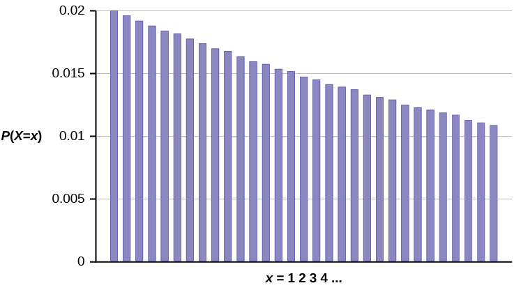
Figure 4.2
The y-axis contains the probability of x, where X = the number of computer components tested. Notice that the probabilities decline by a common increment. This increment is the same ratio between each number and is called a geometric progression and thus the name for this probability density function.
The number of components that you would expect to test until you find the first defective component is the mean,
µ = 50 .
The formula for the mean for the random variable defined as number of failures until first success is μ = 1p =
1 = 50
0.02
See Example 4.9 for an example where the geometric random variable is defined as number of trials until first success. The expected value of this formula for the geometric will be different from this version of the distribution.
The formula for the variance is σ2 = ⎛1 ⎞⎛1 − 1⎞ = ⎛ 1 ⎞⎛ 1 − 1⎞ = 2,450
⎝ p⎠⎝ p
⎠⎝0.02⎠⎝0.02⎠
The standard deviation is σ =
= ⎛ 1 ⎞⎛ 1 − 1⎞ = 49.5
⎛1 ⎞⎛1 − 1⎞⎝ p⎠⎝ p⎠
⎝0.02⎠⎝0.02⎠
Example 4.9The lifetime risk of developing pancreatic cancer is about one in 78 (1.28%). Let X = the number of people you ask before one says he or she has pancreatic cancer. The random variable X in this case includes only the number of trials that were failures and does not count the trial that was a success in finding a person who had the disease.variable with a geometric distribution: X ~ G ⎛ 1 ⎞ or X ~ G(0.0128).The appropriate formula for this random variable is the second one presented above. Then X is a discrete randoma.b.c.⎝78⎠What is the probability of that you ask 9 people before one says he or she has pancreatic cancer? This is asking, what is the probability that you ask 9 people unsuccessfully and the tenth person is a success?What is the probability that you must ask 20 people? Find the (i) mean and (ii) standard deviation of X.
This OpenStax book is available for free at http://cnx.org/content/col11776/1.33
Solution 4.9
a. P(x = 9) = (1 – 0.0128)9 * 0.0128 = 0.0114
b. P(x = 20) = (1 – 0.0128)19 * 0.0128 =0.01
1 − p(1 − 0.0128)
⎛⎞
c.i. Mean = μ === 77.12
⎝⎠
p0.0128
- 1 − p p2
1 − 0.01280.01282
Standard Deviation = σ ==≈ 77.62
4.9 The literacy rate for a nation measures the proportion of people age 15 and over who can read and write. The literacy rate for women in The United Colonies of Independence is 12%. Let X = the number of women you ask until one says that she is literate.What is the probability distribution of X?What is the probability that you ask five women before one says she is literate?What is the probability that you must ask ten women?
Example 4.10A baseball player has a batting average of 0.320. This is the general probability that he gets a hit each time he is at bat.What is the probability that he gets his first hit in the third trip to bat?Solution 4.10P (x=3) = (1-0.32)3-1 × .32 = 0.1480In this case the sequence is failure, failure success.How many trips to bat do you expect the hitter to need before getting a hit?Solution 4.100.320This is simply the expected value of successes and therefore the mean of the distribution.µ = 1p = 1 = 3.125 ≈ 3
Example 4.11There is an 80% chance that a Dalmatian dog has 13 black spots. You go to a dog show and count the spots on Dalmatians. What is the probability that you will review the spots on 3 dogs before you find one that has 13 black spots?Solution 4.11P(x=3) = (1 – 0.80)3 × 0.80 = 0.0064
| Poisson Distribution
Another useful probability distribution is the Poisson distribution, or waiting time distribution. This distribution is used to determine how many checkout clerks are needed to keep the waiting time in line to specified levels, how may telephone lines are needed to keep the system from overloading, and many other practical applications. A modification of the Poisson, the Pascal, invented nearly four centuries ago, is used today by telecommunications companies worldwide for load factors, satellite hookup levels and Internet capacity problems. The distribution gets its name from Simeon Poisson who presented it in 1837 as an extension of the binomial distribution which we will see can be estimated with the Poisson.
There are two main characteristics of a Poisson experiment.
- The Poisson probability distribution gives the probability of a number of events occurring in a fixed interval of time or space if these events happen with a known average rate.
- The events are independently of the time since the last event. For example, a book editor might be interested in the number of words spelled incorrectly in a particular book. It might be that, on the average, there are five words spelled incorrectly in 100 pages. The interval is the 100 pages and it is assumed that there is no relationship between when misspellings occur.
- The random variable X = the number of occurrences in the interval of interest.
Example 4.12A bank expects to receive six bad checks per day, on average. What is the probability of the bank getting fewer than five bad checks on any given day? Of interest is the number of checks the bank receives in one day, so the time interval of interest is one day. Let X = the number of bad checks the bank receives in one day. If the bank expects to receive six bad checks per day then the average is six checks per day. Write a mathematical statement for the probability question.Solution 4.12P(x < 5)
Example 4.13You notice that a news reporter says “uh,” on average, two times per broadcast. What is the probability that the news reporter says “uh” more than two times per broadcast.This is a Poisson problem because you are interested in knowing the number of times the news reporter says “uh” during a broadcast.a. What is the interval of interest?Solution 4.13one broadcast measured in minutesWhat is the average number of times the news reporter says “uh” during one broadcast?Solution 4.132Let X = . What values does X take on?Solution 4.13c. Let X = the number of times the news reporter says “uh” during one broadcast.x = 0, 1, 2, 3, …
This OpenStax book is available for free at http://cnx.org/content/col11776/1.33
d. The probability question is P( ).
Solution 4.13
- P(x > 2)
Notation for the Poisson: P = Poisson Probability Distribution Function
X ~ P(μ)
Read this as “X is a random variable with a Poisson distribution.” The parameter is μ (or λ); μ (or λ) = the mean for the interval of interest. The mean is the number of occurrences that occur on average during the interval period.
The formula for computing probabilities that are from a Poisson process is:
x !
P(x) = µx e– µ
where P(X) is the probability of X successes, μ is the expected number of successes based upon historical data, e is the natural logarithm approximately equal to 2.718, and X is the number of successes per unit, usually per unit of time.
In order to use the Poisson distribution, certain assumptions must hold. These are: the probability of a success, μ, is unchanged within the interval, there cannot be simultaneous successes within the interval, and finally, that the probability of a success among intervals is independent, the same assumption of the binomial distribution.
In a way, the Poisson distribution can be thought of as a clever way to convert a continuous random variable, usually time, into a discrete random variable by breaking up time into discrete independent intervals. This way of thinking about the Poisson helps us understand why it can be used to estimate the probability for the discrete random variable from the binomial distribution. The Poisson is asking for the probability of a number of successes during a period of time while the binomial is asking for the probability of a certain number of successes for a given number of trials.
Example 4.14Leah’s answering machine receives about six telephone calls between 8 a.m. and 10 a.m. What is the probability that Leah receives more than one call in the next 15 minutes?Let X = the number of calls Leah receives in 15 minutes. (The interval of interest is 15 minutes orhour.)14x = 0, 1, 2, 3, …If Leah receives, on the average, six telephone calls in two hours, and there are eight 15 minute intervals in two hours, then Leah receives⎝8⎠X ~ P(0.75)Find P(x > 1). P(x > 1) = 0.1734Probability that Leah receives more than one telephone call in the next 15 minutes is about 0.1734. The graph of X ~ P(0.75) is:⎛1⎞ (6) = 0.75 calls in 15 minutes, on average. So, μ = 0.75 for this problem.
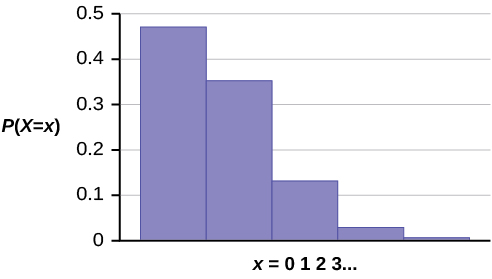
Figure 4.3
The y-axis contains the probability of x where X = the number of calls in 15 minutes.
Example 4.15According to a survey a university professor gets, on average, 7 emails per day. Let X = the number of emails a professor receives per day. The discrete random variable X takes on the values x = 0, 1, 2 …. The random variable X has a Poisson distribution: X ~ P(7). The mean is 7 emails.What is the probability that an email user receives exactly 2 emails per day?What is the probability that an email user receives at most 2 emails per day?What is the standard deviation?Solution 4.15a.P x = 2 =⎛⎞⎝⎠µ ex!x -µ=7 e2 -72!= 0.022b. P x ≤ 2 =⎛⎝⎞⎠7 e0 -70!+7 e1 -71!+7 e2 -72!= 0.029c. Standard Deviation = σ = µ = 7 ≈ 2.65
Example 4.16Text message users receive or send an average of 41.5 text messages per day.How many text messages does a text message user receive or send per hour?What is the probability that a text message user receives or sends two messages per hour?What is the probability that a text message user receives or sends more than two messages per hour?Solution 4.16a. Let X = the number of texts that a user sends or receives in one hour. The average number of texts receivedper hour is41.524≈ 1.7292.
This OpenStax book is available for free at http://cnx.org/content/col11776/1.33
b. P⎛x = 2⎞ = µx e-µ = 1.7292 e-1.729 = 0.265
⎝⎠x!2!
c.P⎛x > 2⎞ = 1 – P⎛x ≤ 2⎞ = 1 – ⎡70 e-7 + 71 e-7 + 72 e-7⎤ = 0.250
⎝⎠⎝⎠⎣ 0!1!2! ⎦
Example 4.17On May 13, 2013, starting at 4:30 PM, the probability of low seismic activity for the next 48 hours in Alaska was reported as about 1.02%. Use this information for the next 200 days to find the probability that there will be low seismic activity in ten of the next 200 days. Use both the binomial and Poisson distributions to calculate the probabilities. Are they close?Solution 4.17Let X = the number of days with low seismic activity. Using the binomial distribution:• P⎛x = 10⎞ =⎝⎠10!(200 – 10)!200!×.010210 = 0.000039Using the Poisson distribution:• Calculate μ = np = 200(0.0102) ≈ 2.04• P x = 10 =⎛⎝⎞µ e⎠x -µx!=2.04e10 -2.0410!= 0.000045We expect the approximation to be good because n is large (greater than 20) and p is small (less than 0.05). The results are close—both probabilities reported are almost 0.
Estimating the Binomial Distribution with the Poisson Distribution
We found before that the binomial distribution provided an approximation for the hypergeometric distribution. Now we find that the Poisson distribution can provide an approximation for the binomial. We say that the binomial distribution approaches the Poisson. The binomial distribution approaches the Poisson distribution is as n gets larger and p is small such that np becomes a constant value. There are several rules of thumb for when one can say they will use a Poisson to estimate a binomial. One suggests that np, the mean of the binomial, should be less than 25. Another author suggests that it should be less than 7. And another, noting that the mean and variance of the Poisson are both the same, suggests that np and npq, the mean and variance of the binomial, should be greater than 5. There is no one broadly accepted rule of thumb for when one can use the Poisson to estimate the binomial.
As we move through these probability distributions we are getting to more sophisticated distributions that, in a sense, contain the less sophisticated distributions within them. This proposition has been proven by mathematicians. This gets us to the highest level of sophistication in the next probability distribution which can be used as an approximation to all of those that we have discussed so far. This is the normal distribution.
Example 4.18A survey of 500 seniors in the Price Business School yields the following information. 75% go straight to work after graduation. 15% go on to work on their MBA. 9% stay to get a minor in another program. 1% go on to get a Master’s in Finance.What is the probability that more than 2 seniors go to graduate school for their Master’s in finance?
Solution 4.18
This is clearly a binomial probability distribution problem. The choices are binary when we define the results as “Graduate School in Finance” versus “all other options.” The random variable is discrete, and the events are, we could assume, independent. Solving as a binomial problem, we have:
Binomial Solution
n * p = 500 * 0.01 = 5 = µ
0 !(500 − 0)!
P(0) = 500 !0.010(1 − 0.01)500−0 = 0.00657
1 !(500 − 1)!
P(1) = 500 !0.011(1 − 0.01)500−1 = 0.03318
2 !(500 − 2)!
P(2) = 500 !0.012(1 − 0.01)500−2 = 0.08363
Adding all 3 together = 0.12339
Poisson approximation
1 − 0.12339 = 0.87661
n * p = 500 * 0.01 = 5 = µ
n * p * (1 − p) = 500 * 0.01 * ⎛0.99⎞ ≈ 5 = σ 2 = µ
⎩
e−np(np) x⎧
⎝
⎭
⎩
e−5 * 50⎫⎧
⎠
⎭
⎩
e−5 * 51⎫⎧
e−5 * 52⎫
P(X) =
x != ⎨P(0) =
0 !⎬ + ⎨P(1) =
1 !⎬ + ⎨P(2) =
2 !⎬
⎭
0.0067 + 0.0337 + 0.0842 = 0.1247
1 − 0.1247 = 0.8753
An approximation that is off by 1 one thousandth is certainly an acceptable approximation.
This OpenStax book is available for free at http://cnx.org/content/col11776/1.33
Bernoulli Trials an experiment with the following characteristics:
- There are only two possible outcomes called “success” and “failure” for each trial.
- The probability p of a success is the same for any trial (so the probability q = 1 − p of a failure is the same for any trial).
Binomial Experiment a statistical experiment that satisfies the following three conditions:
- There are a fixed number of trials, n.
- There are only two possible outcomes, called “success” and, “failure,” for each trial. The letter p denotes the probability of a success on one trial, and q denotes the probability of a failure on one trial.
- The n trials are independent and are repeated using identical conditions.
standard deviation is σ = npq . The probability of exactly x successes in n trials is
⎝x⎠
P(X = x) = ⎛n⎞ pxqn − x.
μ = 1 and the standard deviation is σ =1 ⎛1 − 1⎞ . The probability of exactly x failures before the first success is
pp⎝ p⎠
given by the formula: P(X = x) = p(1 – p)x – 1 where one wants to know probability for the number of trials until the first success: the xth trail is the first success.
An alternative formulation of the geometric distribution asks the question: what is the probability of x failures until the first success? In this formulation the trial that resulted in the first success is not counted. The formula for this
presentation of the geometric is: P(X = x) = p(1 − p) x
p
The expected value in this form of the geometric distribution is µ = 1 − p
The easiest way to keep these two forms of the geometric distribution straight is to remember that p is the probability of success and (1−p) is the probability of failure. In the formula the exponents simply count the number of successes and number of failures of the desired outcome of the experiment. Of course the sum of these two numbers must add to the number of trials in the experiment.
Geometric Experiment a statistical experiment with the following properties:
- There are one or more Bernoulli trials with all failures except the last one, which is a success.
- In theory, the number of trials could go on forever. There must be at least one trial.
- The probability, p, of a success and the probability, q, of a failure do not change from trial to trial.
Hypergeometric Experiment a statistical experiment with the following properties:
- You take samples from two groups.
- You are concerned with a group of interest, called the first group.
- You sample without replacement from the combined groups.
- Each pick is not independent, since sampling is without replacement.
Hypergeometric Probability a discrete random variable (RV) that is characterized by:
- A fixed number of trials.
- The probability of success is not the same from trial to trial.
We sample from two groups of items when we are interested in only one group. X is defined as the number of successes out of the total number of items chosen.
- The probability that the event occurs in a given interval is the same for all intervals.
- The events occur with a known mean and independently of the time since the last event.
The distribution is defined by the mean μ of the event in the interval. The mean is μ = np. The standard deviation
is σ = µ
. The probability of having exactly x successes in r trials is
µx e– µ
P(x) =
x !. The Poisson distribution is
often used to approximate the binomial distribution, when n is “large” and p is “small” (a general rule is that np
should be greater than or equal to 25 and p should be less than or equal to 0.01).
- The domain of the random variable (RV) is not necessarily a numerical set; the domain may be expressed in words; for example, if X = hair color then the domain is {black, blond, gray, green, orange}.
- We can tell what specific value x the random variable X takes only after performing the experiment.
CHAPTER REVIEW
The characteristics of a probability distribution or density function (PDF) are as follows:
- Each probability is between zero and one, inclusive (inclusive means to include zero and one).
- The sum of the probabilities is one.
The combinatorial formula can provide the number of unique subsets of size x that can be created from n unique objects to
⎝x⎠
help us calculate probabilities. The combinatorial formula is ⎛n⎞
n !
= n Cx =
x !(n – x)!
A hypergeometric experiment is a statistical experiment with the following properties:
- You take samples from two groups.
- You are concerned with a group of interest, called the first group.
- You sample without replacement from the combined groups.
- Each pick is not independent, since sampling is without replacement.
The outcomes of a hypergeometric experiment fit a hypergeometric probability distribution. The random variable X = the
A N – A
⎛ ⎞⎛⎞
⎛N⎞
number of items from the group of interest. h(x) = ⎝ x ⎠⎝ n – x ⎠ .
⎝ n ⎠
A statistical experiment can be classified as a binomial experiment if the following conditions are met:
- There are a fixed number of trials, n.
- There are only two possible outcomes, called “success” and, “failure” for each trial. The letter p denotes the
This OpenStax book is available for free at http://cnx.org/content/col11776/1.33
probability of a success on one trial and q denotes the probability of a failure on one trial.
- The n trials are independent and are repeated using identical conditions.
The outcomes of a binomial experiment fit a binomial probability distribution. The random variable X = the number of successes obtained in the n independent trials. The mean of X can be calculated using the formula μ = np, and the standard deviation is given by the formula σ = npq .
The formula for the Binomial probability density function is
n –
P(x) = x !( n ! x)! · px q(n – x)
There are three characteristics of a geometric experiment:
- There are one or more Bernoulli trials with all failures except the last one, which is a success.
- In theory, the number of trials could go on forever. There must be at least one trial.
- The probability, p, of a success and the probability, q, of a failure are the same for each trial.
In a geometric experiment, define the discrete random variable X as the number of independent trials until the first success. We say that X has a geometric distribution and write X ~ G(p) where p is the probability of success in a single trial.
The mean of the geometric distribution X ~ G(p) is μ = 1 / p where x = number of trials until first success for the formula
P(X = x) = (1 – p) x – 1 p where the number of trials is up and including the first success.
An alternative formulation of the geometric distribution asks the question: what is the probability of x failures until the first success? In this formulation the trial that resulted in the first success is not counted. The formula for this presentation of the geometric is:
P(X = x) = p(1 − p) x
The expected value in this form of the geometric distribution is
p
µ = 1 − p
The easiest way to keep these two forms of the geometric distribution straight is to remember that p is the probability of success and (1−p) is the probability of failure. In the formula the exponents simply count the number of successes and number of failures of the desired outcome of the experiment. Of course the sum of these two numbers must add to the number of trials in the experiment.
The formula for computing probabilities that are from a Poisson process is:
x !
P(x) = µx e– µ
where P(X) is the probability of successes, μ (pronounced mu) is the expected number of successes, e is the natural logarithm approximately equal to 2.718, and X is the number of successes per unit, usually per unit of time.
FORMULA REVIEW
A N – A
⎛ ⎞⎛⎞
⎛N⎞
h(x) = ⎝ x ⎠⎝ n – x ⎠
⎝ n ⎠
X ~ B(n, p) means that the discrete random variable X has a binomial probability distribution with n trials and probability of success p.
X = the number of successes in n independent trials
n = the number of independent trials
X takes on the values x = 0, 1, 2, 3, …, n
p = the probability of a success for any trial q = the probability of a failure for any trial p + q = 1
q = 1 – p
The mean of X is μ = np. The standard deviation of X is σ =
npq .
n –
P(x) = x !( n ! x)! · px q(n – x)
where P(X) is the probability of X successes in n trials when the probability of a success in ANY ONE TRIAL is p.
P(X = x) = p(1 − p) x − 1
X ~ G(p) means that the discrete random variable X has a geometric probability distribution with probability of success in a single trial p.
X = the number of independent trials until the first success
X takes on the values x = 1, 2, 3, …
p = the probability of a success for any trial
q = the probability of a failure for any trial p + q = 1
q = 1 – p
1 – p p2
1p⎛1p − 1⎞⎝⎠
The mean is μ = 1p .
The standard deviation is σ ==.
X ~ P(μ) means that X has a Poisson probability distribution where X = the number of occurrences in the interval of interest.
X takes on the values x = 0, 1, 2, 3, … The mean μ or λ is typically given.
The variance is σ2 = μ, and the standard deviation is
σ = µ .
When P(μ) is used to approximate a binomial distribution, μ = np where n represents the number of independent trials and p represents the probability of success in a single trial.
x !
P(x) = µx e– µ
PRACTICE
Use the following information to answer the next five exercises: A company wants to evaluate its attrition rate, in other words, how long new hires stay with the company. Over the years, they have established the following probability distribution.
Let X = the number of years a new hire will stay with the company.
Let P(x) = the probability that a new hire will stay with the company x years.
This OpenStax book is available for free at http://cnx.org/content/col11776/1.33
1. Complete Table 4.1 using the data provided.
|
P(x) |
|
|
0 |
0.12 |
|
1 |
0.18 |
|
2 |
0.30 |
|
3 |
0.15 |
|
4 |
|
|
5 |
0.10 |
|
6 |
0.05 |
Table 4.1
2. P(x = 4) =
- On average, how long would you expect a new hire to stay with the company?
- What does the column “P(x)” sum to?
Use the following information to answer the next six exercises: A baker is deciding how many batches of muffins to make to sell in his bakery. He wants to make enough to sell every one and no fewer. Through observation, the baker has established a probability distribution.
|
x |
P(x) |
|
1 |
0.15 |
|
2 |
0.35 |
|
3 |
0.40 |
|
4 |
0.10 |
Table 4.2
- Define the random variable X.
- What is the probability the baker will sell more than one batch? P(x > 1) =
- What is the probability the baker will sell exactly one batch? P(x = 1) =
- On average, how many batches should the baker make?
Use the following information to answer the next four exercises: Ellen has music practice three days a week. She practices for all of the three days 85% of the time, two days 8% of the time, one day 4% of the time, and no days 3% of the time. One week is selected at random.
- Define the random variable X.
- Construct a probability distribution table for the data.
- We know that for a probability distribution function to be discrete, it must have two characteristics. One is that the sum of the probabilities is one. What is the other characteristic?
Use the following information to answer the next five exercises: Javier volunteers in community events each month. He does not do more than five events in a month. He attends exactly five events 35% of the time, four events 25% of the time,
three events 20% of the time, two events 10% of the time, one event 5% of the time, and no events 5% of the time.
- Define the random variable X.
- What values does x take on?
- Construct a PDF table.
- Find the probability that Javier volunteers for less than three events each month. P(x < 3) =
- Find the probability that Javier volunteers for at least one event each month. P(x > 0) =
Use the following information to answer the next five exercises: Suppose that a group of statistics students is divided into two groups: business majors and non-business majors. There are 16 business majors in the group and seven non-business majors in the group. A random sample of nine students is taken. We are interested in the number of business majors in the sample.
Use the following information to answer the next eight exercises: The Higher Education Research Institute at UCLA collected data from 203,967 incoming first-time, full-time freshmen from 270 four-year colleges and universities in the U.S. 71.3% of those students replied that, yes, they believe that same-sex couples should have the right to legal marital status. Suppose that you randomly pick eight first-time, full-time freshmen from the survey. You are interested in the number that believes that same sex-couples should have the right to legal marital status.
21. X ~ ( ,)
- What values does the random variable X take on?
- Construct the probability distribution function (PDF).
|
x |
P(x) |
|
|
|
|
|
|
|
|
|
|
|
|
|
|
|
|
|
|
|
|
|
|
|
|
|
|
|
Table 4.3
- On average (μ), how many would you expect to answer yes?
- What is the standard deviation (σ)?
- What is the probability that at most five of the freshmen reply “yes”?
- What is the probability that at least two of the freshmen reply “yes”?
Use the following information to answer the next six exercises: The Higher Education Research Institute at UCLA collected
This OpenStax book is available for free at http://cnx.org/content/col11776/1.33
data from 203,967 incoming first-time, full-time freshmen from 270 four-year colleges and universities in the U.S. 71.3% of those students replied that, yes, they believe that same-sex couples should have the right to legal marital status. Suppose that you randomly select freshman from the study until you find one who replies “yes.” You are interested in the number of freshmen you must ask.
29. X ~ ( ,)
- What values does the random variable X take on?
- Construct the probability distribution function (PDF). Stop at x = 6.
|
x |
P(x) |
|
1 |
|
|
2 |
|
|
3 |
|
|
4 |
|
|
5 |
|
|
6 |
|
Table 4.4
- On average (μ), how many freshmen would you expect to have to ask until you found one who replies “yes?”
- What is the probability that you will need to ask fewer than three freshmen?
Use the following information to answer the next six exercises: On average, a clothing store gets 120 customers per day.
- Assume the event occurs independently in any given day. Define the random variable X.
- What values does X take on?
- What is the probability of getting 150 customers in one day?
- What is the probability of getting 35 customers in the first four hours? Assume the store is open 12 hours each day.
- What is the probability that the store will have more than 12 customers in the first hour?
- What is the probability that the store will have fewer than 12 customers in the first two hours?
- Which type of distribution can the Poisson model be used to approximate? When would you do this?
Use the following information to answer the next six exercises: On average, eight teens in the U.S. die from motor vehicle injuries per day. As a result, states across the country are debating raising the driving age.
42. X ~ ( ,)
- What values does X take on?
- For the given values of the random variable X, fill in the corresponding probabilities.
- Is it likely that there will be no teens killed from motor vehicle injuries on any given day in the U.S? Justify your answer numerically.
- Is it likely that there will be more than 20 teens killed from motor vehicle injuries on any given day in the U.S.? Justify your answer numerically.
HOMEWORK
- A group of Martial Arts students is planning on participating in an upcoming demonstration. Six are students of Tae Kwon Do; seven are students of Shotokan Karate. Suppose that eight students are randomly picked to be in the first demonstration. We are interested in the number of Shotokan Karate students in that first demonstration.
- In words, define the random variable X.
- List the values that X may take on.
- How many Shotokan Karate students do we expect to be in that first demonstration?
- In one of its Spring catalogs, L.L. Bean® advertised footwear on 29 of its 192 catalog pages. Suppose we randomly survey 20 pages. We are interested in the number of pages that advertise footwear. Each page may be picked at most once.
- In words, define the random variable X.
- List the values that X may take on.
- How many pages do you expect to advertise footwear on them?
- Calculate the standard deviation.
- Suppose that a technology task force is being formed to study technology awareness among instructors. Assume that ten people will be randomly chosen to be on the committee from a group of 28 volunteers, 20 who are technically proficient and eight who are not. We are interested in the number on the committee who are not technically proficient.
- In words, define the random variable X.
- List the values that X may take on.
- How many instructors do you expect on the committee who are not technically proficient?
- Find the probability that at least five on the committee are not technically proficient.
- Find the probability that at most three on the committee are not technically proficient.
- Suppose that nine Massachusetts athletes are scheduled to appear at a charity benefit. The nine are randomly chosen from eight volunteers from the Boston Celtics and four volunteers from the New England Patriots. We are interested in the number of Patriots picked.
- In words, define the random variable X.
- List the values that X may take on.
- Are you choosing the nine athletes with or without replacement?
- A bridge hand is defined as 13 cards selected at random and without replacement from a deck of 52 cards. In a standard deck of cards, there are 13 cards from each suit: hearts, spades, clubs, and diamonds. What is the probability of being dealt a hand that does not contain a heart?
- What is the group of interest?
- How many are in the group of interest?
- How many are in the other group?
- Let X = . What values does X take on?
- The probability question is P( ).
- Find the probability in question.
- Find the (i) mean and (ii) standard deviation of X.
- According to a recent article the average number of babies born with significant hearing loss (deafness) is approximately two per 1,000 babies in a healthy baby nursery. The number climbs to an average of 30 per 1,000 babies in an intensive care nursery.
Suppose that 1,000 babies from healthy baby nurseries were randomly surveyed. Find the probability that exactly two babies were born deaf.
Use the following information to answer the next four exercises. Recently, a nurse commented that when a patient calls the medical advice line claiming to have the flu, the chance that he or she truly has the flu (and not just a nasty cold) is only about 4%. Of the next 25 patients calling in claiming to have the flu, we are interested in how many actually have the flu.
- Define the random variable and list its possible values.
- State the distribution of X.
- Find the probability that at least four of the 25 patients actually have the flu.
This OpenStax book is available for free at http://cnx.org/content/col11776/1.33
- On average, for every 25 patients calling in, how many do you expect to have the flu?
- People visiting video rental stores often rent more than one DVD at a time. The probability distribution for DVD rentals per customer at Video To Go is given Table 4.5. There is five-video limit per customer at this store, so nobody ever rents more than five DVDs.
|
P(x) |
|
|
0 |
0.03 |
|
1 |
0.50 |
|
2 |
0.24 |
|
3 |
|
|
4 |
0.07 |
|
5 |
0.04 |
Table 4.5
- Describe the random variable X in words.
- Find the probability that a customer rents three DVDs.
- Find the probability that a customer rents at least four DVDs.
- Find the probability that a customer rents at most two DVDs.
- A school newspaper reporter decides to randomly survey 12 students to see if they will attend Tet (Vietnamese New Year) festivities this year. Based on past years, she knows that 18% of students attend Tet festivities. We are interested in the number of students who will attend the festivities.
- In words, define the random variable X.
- List the values that X may take on.
- Give the distribution of X. X ~ ( ,)
- How many of the 12 students do we expect to attend the festivities?
- Find the probability that at most four students will attend.
- Find the probability that more than two students will attend.
Use the following information to answer the next two exercises: The probability that the San Jose Sharks will win any given game is 0.3694 based on a 13-year win history of 382 wins out of 1,034 games played (as of a certain date). An upcoming monthly schedule contains 12 games.
b. 12
c.382 1043
d. 4.43
Let X = the number of games won in that upcoming month.
- What is the probability that the San Jose Sharks win six games in that upcoming month? a. 0.1476
b. 0.2336
c. 0.7664
d. 0.8903
- What is the probability that the San Jose Sharks win at least five games in that upcoming month a. 0.3694
b. 0.5266
c. 0.4734
d. 0.2305
- A student takes a ten-question true-false quiz, but did not study and randomly guesses each answer. Find the probability that the student passes the quiz with a grade of at least 70% of the questions correct.
- A student takes a 32-question multiple-choice exam, but did not study and randomly guesses each answer. Each question has three possible choices for the answer. Find the probability that the student guesses more than 75% of the questions correctly.
- Six different colored dice are rolled. Of interest is the number of dice that show a one.
- In words, define the random variable X.
- List the values that X may take on.
- On average, how many dice would you expect to show a one?
- Find the probability that all six dice show a one.
- Is it more likely that three or that four dice will show a one? Use numbers to justify your answer numerically.
- More than 96 percent of the very largest colleges and universities (more than 15,000 total enrollments) have some online offerings. Suppose you randomly pick 13 such institutions. We are interested in the number that offer distance learning courses.
- In words, define the random variable X.
- List the values that X may take on.
- Give the distribution of X. X ~ ( ,)
- On average, how many schools would you expect to offer such courses?
- Find the probability that at most ten offer such courses.
- Is it more likely that 12 or that 13 will offer such courses? Use numbers to justify your answer numerically and answer in a complete sentence.
- Suppose that about 85% of graduating students attend their graduation. A group of 22 graduating students is randomly chosen.
- In words, define the random variable X.
- List the values that X may take on.
- Give the distribution of X. X ~ ( ,)
- How many are expected to attend their graduation?
- Find the probability that 17 or 18 attend.
- Based on numerical values, would you be surprised if all 22 attended graduation? Justify your answer numerically.
- At The Fencing Center, 60% of the fencers use the foil as their main weapon. We randomly survey 25 fencers at The Fencing Center. We are interested in the number of fencers who do not use the foil as their main weapon.
- In words, define the random variable X.
- List the values that X may take on.
- Give the distribution of X. X ~ ( ,)
- How many are expected to not to use the foil as their main weapon?
- Find the probability that six do not use the foil as their main weapon.
- Based on numerical values, would you be surprised if all 25 did not use foil as their main weapon? Justify your answer numerically.
- Approximately 8% of students at a local high school participate in after-school sports all four years of high school. A group of 60 seniors is randomly chosen. Of interest is the number who participated in after-school sports all four years of high school.
- In words, define the random variable X.
- List the values that X may take on.
- Give the distribution of X. X ~ ( ,)
- How many seniors are expected to have participated in after-school sports all four years of high school?
- Based on numerical values, would you be surprised if none of the seniors participated in after-school sports all four years of high school? Justify your answer numerically.
- Based upon numerical values, is it more likely that four or that five of the seniors participated in after-school sports all four years of high school? Justify your answer numerically.
- The chance of an IRS audit for a tax return with over $25,000 in income is about 2% per year. We are interested in the expected number of audits a person with that income has in a 20-year period. Assume each year is independent.
- In words, define the random variable X.
- List the values that X may take on.
- Give the distribution of X. X ~ ( ,)
- How many audits are expected in a 20-year period?
- Find the probability that a person is not audited at all.
- Find the probability that a person is audited more than twice.
This OpenStax book is available for free at http://cnx.org/content/col11776/1.33
- It has been estimated that only about 30% of California residents have adequate earthquake supplies. Suppose you randomly survey 11 California residents. We are interested in the number who have adequate earthquake supplies.
- In words, define the random variable X.
- List the values that X may take on.
- Give the distribution of X. X ~ ( ,)
- What is the probability that at least eight have adequate earthquake supplies?
- Is it more likely that none or that all of the residents surveyed will have adequate earthquake supplies? Why?
- How many residents do you expect will have adequate earthquake supplies?
- There are two similar games played for Chinese New Year and Vietnamese New Year. In the Chinese version, fair dice with numbers 1, 2, 3, 4, 5, and 6 are used, along with a board with those numbers. In the Vietnamese version, fair dice with pictures of a gourd, fish, rooster, crab, crayfish, and deer are used. The board has those six objects on it, also. We will play with bets being $1. The player places a bet on a number or object. The “house” rolls three dice. If none of the dice show the number or object that was bet, the house keeps the $1 bet. If one of the dice shows the number or object bet (and the other two do not show it), the player gets back his or her $1 bet, plus $1 profit. If two of the dice show the number or object bet (and the third die does not show it), the player gets back his or her $1 bet, plus $2 profit. If all three dice show the number or object bet, the player gets back his or her $1 bet, plus $3 profit. Let X = number of matches and Y = profit per game.
- In words, define the random variable X.
- List the values that X may take on.
- List the values that Y may take on. Then, construct one PDF table that includes both X and Y and their probabilities.
- Calculate the average expected matches over the long run of playing this game for the player.
- Calculate the average expected earnings over the long run of playing this game for the player.
- Determine who has the advantage, the player or the house.
- According to The World Bank, only 9% of the population of Uganda had access to electricity as of 2009. Suppose we randomly sample 150 people in Uganda. Let X = the number of people who have access to electricity.
- What is the probability distribution for X?
- Using the formulas, calculate the mean and standard deviation of X.
- Find the probability that 15 people in the sample have access to electricity.
- Find the probability that at most ten people in the sample have access to electricity.
- Find the probability that more than 25 people in the sample have access to electricity.
- The literacy rate for a nation measures the proportion of people age 15 and over that can read and write. The literacy rate in Afghanistan is 28.1%. Suppose you choose 15 people in Afghanistan at random. Let X = the number of people who are literate.
- Sketch a graph of the probability distribution of X.
- Using the formulas, calculate the (i) mean and (ii) standard deviation of X.
- Find the probability that more than five people in the sample are literate. Is it is more likely that three people or four people are literate.
- A consumer looking to buy a used red Miata car will call dealerships until she finds a dealership that carries the car. She estimates the probability that any independent dealership will have the car will be 28%. We are interested in the number of dealerships she must call.
- In words, define the random variable X.
- List the values that X may take on.
- Give the distribution of X. X ~ ( ,)
- On average, how many dealerships would we expect her to have to call until she finds one that has the car?
- Find the probability that she must call at most four dealerships.
- Find the probability that she must call three or four dealerships.
- Suppose that the probability that an adult in America will watch the Super Bowl is 40%. Each person is considered independent. We are interested in the number of adults in America we must survey until we find one who will watch the Super Bowl.
- In words, define the random variable X.
- List the values that X may take on.
- Give the distribution of X. X ~ ( ,)
- How many adults in America do you expect to survey until you find one who will watch the Super Bowl?
- Find the probability that you must ask seven people.
- Find the probability that you must ask three or four people.
- It has been estimated that only about 30% of California residents have adequate earthquake supplies. Suppose we are interested in the number of California residents we must survey until we find a resident who does not have adequate earthquake supplies.
- In words, define the random variable X.
- List the values that X may take on.
- Give the distribution of X. X ~ ( ,)
- What is the probability that we must survey just one or two residents until we find a California resident who does not have adequate earthquake supplies?
- What is the probability that we must survey at least three California residents until we find a California resident who does not have adequate earthquake supplies?
- How many California residents do you expect to need to survey until you find a California resident who does not
have adequate earthquake supplies?
- How many California residents do you expect to need to survey until you find a California resident who does
have adequate earthquake supplies?
- In one of its Spring catalogs, L.L. Bean® advertised footwear on 29 of its 192 catalog pages. Suppose we randomly survey 20 pages. We are interested in the number of pages that advertise footwear. Each page may be picked more than once.
- In words, define the random variable X.
- List the values that X may take on.
- Give the distribution of X. X ~ ( ,)
- How many pages do you expect to advertise footwear on them?
- Is it probable that all twenty will advertise footwear on them? Why or why not?
- What is the probability that fewer than ten will advertise footwear on them?
- Reminder: A page may be picked more than once. We are interested in the number of pages that we must randomly survey until we find one that has footwear advertised on it. Define the random variable X and give its distribution.
- What is the probability that you only need to survey at most three pages in order to find one that advertises footwear on it?
- How many pages do you expect to need to survey in order to find one that advertises footwear?
- Suppose that you are performing the probability experiment of rolling one fair six-sided die. Let F be the event of rolling a four or a five. You are interested in how many times you need to roll the die in order to obtain the first four or five as the outcome.
- p = probability of success (event F occurs)
- q = probability of failure (event F does not occur)
- Write the description of the random variable X.
- What are the values that X can take on?
- Find the values of p and q.
- Find the probability that the first occurrence of event F (rolling a four or five) is on the second trial.
- Ellen has music practice three days a week. She practices for all of the three days 85% of the time, two days 8% of the time, one day 4% of the time, and no days 3% of the time. One week is selected at random. What values does X take on?
This OpenStax book is available for free at http://cnx.org/content/col11776/1.33
- The World Bank records the prevalence of HIV in countries around the world. According to their data, “Prevalence of HIV refers to the percentage of people ages 15 to 49 who are infected with HIV.”[1] In South Africa, the prevalence of HIV is 17.3%. Let X = the number of people you test until you find a person infected with HIV.
- Sketch a graph of the distribution of the discrete random variable X.
- What is the probability that you must test 30 people to find one with HIV?
- What is the probability that you must ask ten people?
- Find the (i) mean and (ii) standard deviation of the distribution of X.
- According to a recent Pew Research poll, 75% of millenials (people born between 1981 and 1995) have a profile on a social networking site. Let X = the number of millenials you ask until you find a person without a profile on a social networking site.
- Describe the distribution of X.
- Find the (i) mean and (ii) standard deviation of X.
- What is the probability that you must ask ten people to find one person without a social networking site?
- What is the probability that you must ask 20 people to find one person without a social networking site?
- What is the probability that you must ask at most five people?
- The switchboard in a Minneapolis law office gets an average of 5.5 incoming phone calls during the noon hour on Mondays. Experience shows that the existing staff can handle up to six calls in an hour. Let X = the number of calls received at noon.
- Find the mean and standard deviation of X.
- What is the probability that the office receives at most six calls at noon on Monday?
- Find the probability that the law office receives six calls at noon. What does this mean to the law office staff who get, on average, 5.5 incoming phone calls at noon?
- What is the probability that the office receives more than eight calls at noon?
- The maternity ward at Dr. Jose Fabella Memorial Hospital in Manila in the Philippines is one of the busiest in the world with an average of 60 births per day. Let X = the number of births in an hour.
- Find the mean and standard deviation of X.
- Sketch a graph of the probability distribution of X.
- What is the probability that the maternity ward will deliver three babies in one hour?
- What is the probability that the maternity ward will deliver at most three babies in one hour?
- What is the probability that the maternity ward will deliver more than five babies in one hour?
- A manufacturer of Christmas tree light bulbs knows that 3% of its bulbs are defective. Find the probability that a string of 100 lights contains at most four defective bulbs using both the binomial and Poisson distributions.
- The average number of children a Japanese woman has in her lifetime is 1.37. Suppose that one Japanese woman is randomly chosen.
- In words, define the random variable X.
- List the values that X may take on.
- Find the probability that she has no children.
- Find the probability that she has fewer children than the Japanese average.
- Find the probability that she has more children than the Japanese average.
- The average number of children a Spanish woman has in her lifetime is 1.47. Suppose that one Spanish woman is randomly chosen.
- In words, define the Random Variable X.
- List the values that X may take on.
- Find the probability that she has no children.
- Find the probability that she has fewer children than the Spanish average.
- Find the probability that she has more children than the Spanish average .
1. ”Prevalence of HIV, total (% of populations ages 15-49),” The World Bank, 2013. Available online at http://data.worldbank.org/indicator/ SH.DYN.AIDS.ZS?order=wbapi_data_value_2011+wbapi_data_value+wbapi_data_value-last&sort=desc (accessed May 15, 2013).
- Fertile, female cats produce an average of three litters per year. Suppose that one fertile, female cat is randomly chosen. In one year, find the probability she produces:
- In words, define the random variable X.
- List the values that X may take on.
- Give the distribution of X. X ~
- Find the probability that she has no litters in one year.
- Find the probability that she has at least two litters in one year.
- Find the probability that she has exactly three litters in one year.
- The chance of having an extra fortune in a fortune cookie is about 3%. Given a bag of 144 fortune cookies, we are interested in the number of cookies with an extra fortune. Two distributions may be used to solve this problem, but only use one distribution to solve the problem.
- In words, define the random variable X.
- List the values that X may take on.
- How many cookies do we expect to have an extra fortune?
- Find the probability that none of the cookies have an extra fortune.
- Find the probability that more than three have an extra fortune.
- As n increases, what happens involving the probabilities using the two distributions? Explain in complete sentences.
- According to the South Carolina Department of Mental Health web site, for every 200 U.S. women, the average number who suffer from anorexia is one. Out of a randomly chosen group of 600 U.S. women determine the following.
- In words, define the random variable X.
- List the values that X may take on.
- Give the distribution ofX. X ~ ( ,)
- How many are expected to suffer from anorexia?
- Find the probability that no one suffers from anorexia.
- Find the probability that more than four suffer from anorexia.
- The chance of an IRS audit for a tax return with over $25,000 in income is about 2% per year. Suppose that 100 people with tax returns over $25,000 are randomly picked. We are interested in the number of people audited in one year. Use a Poisson distribution to anwer the following questions.
- In words, define the random variable X.
- List the values that X may take on.
- How many are expected to be audited?
- Find the probability that no one was audited.
- Find the probability that at least three were audited.
- Approximately 8% of students at a local high school participate in after-school sports all four years of high school. A group of 60 seniors is randomly chosen. Of interest is the number that participated in after-school sports all four years of high school.
- In words, define the random variable X.
- List the values that X may take on.
- How many seniors are expected to have participated in after-school sports all four years of high school?
- Based on numerical values, would you be surprised if none of the seniors participated in after-school sports all four years of high school? Justify your answer numerically.
- Based on numerical values, is it more likely that four or that five of the seniors participated in after-school sports all four years of high school? Justify your answer numerically.
- On average, Pierre, an amateur chef, drops three pieces of egg shell into every two cake batters he makes. Suppose that you buy one of his cakes.
- In words, define the random variable X.
- List the values that X may take on.
- On average, how many pieces of egg shell do you expect to be in the cake?
- What is the probability that there will not be any pieces of egg shell in the cake?
- Let’s say that you buy one of Pierre’s cakes each week for six weeks. What is the probability that there will not be any egg shell in any of the cakes?
- Based upon the average given for Pierre, is it possible for there to be seven pieces of shell in the cake? Why?
Use the following information to answer the next two exercises: The average number of times per week that Mrs. Plum’s cats wake her up at night because they want to play is ten. We are interested in the number of times her cats wake her up
This OpenStax book is available for free at http://cnx.org/content/col11776/1.33
each week.
- In words, the random variable X =
- the number of times Mrs. Plum’s cats wake her up each week.
- the number of times Mrs. Plum’s cats wake her up each hour.
- the number of times Mrs. Plum’s cats wake her up each night.
- the number of times Mrs. Plum’s cats wake her up.
- Find the probability that her cats will wake her up no more than five times next week. a. 0.5000
b. 0.9329
c. 0.0378
d. 0.0671
REFERENCES
“Access to electricity (% of population),” The World Bank, 2013. Available online at http://data.worldbank.org/indicator/ EG.ELC.ACCS.ZS?order=wbapi_data_value_2009%20wbapi_data_value%20wbapi_data_value-first&sort=asc (accessed May 15, 2015).
“Distance Education.” Wikipedia. Available online at http://en.wikipedia.org/wiki/Distance_education (accessed May 15, 2013).
“NBA Statistics – 2013,” ESPN NBA, 2013. Available online at http://espn.go.com/nba/statistics/_/seasontype/2 (accessed May 15, 2013).
Newport, Frank. “Americans Still Enjoy Saving Rather than Spending: Few demographic differences seen in these views other than by income,” GALLUP® Economy, 2013. Available online at http://www.gallup.com/poll/162368/americans- enjoy-saving-rather-spending.aspx (accessed May 15, 2013).
Pryor, John H., Linda DeAngelo, Laura Palucki Blake, Sylvia Hurtado, Serge Tran. The American Freshman: National Norms Fall 2011. Los Angeles: Cooperative Institutional Research Program at the Higher Education Research Institute at UCLA, 2011. Also available online at http://heri.ucla.edu/PDFs/pubs/TFS/Norms/Monographs/ TheAmericanFreshman2011.pdf (accessed May 15, 2013).
“The World FactBook,” Central Intelligence Agency. Available online at https://www.cia.gov/library/publications/the- world-factbook/geos/af.html (accessed May 15, 2013).
“What are the key statistics about pancreatic cancer?” American Cancer Society, 2013. Available online at http://www.cancer.org/cancer/pancreaticcancer/detailedguide/pancreatic-cancer-key-statistics (accessed May 15, 2013).
“Millennials: A Portrait of Generation Next,” PewResearchCenter. Available online at http://www.pewsocialtrends.org/ files/2010/10/millennials-confident-connected-open-to-change.pdf (accessed May 15, 2013).
“Millennials: Confident. Connected. Open to Change.” Executive Summary by PewResearch Social & Demographic Trends, 2013. Available online at http://www.pewsocialtrends.org/2010/02/24/millennials-confident-connected-open-to- change/ (accessed May 15, 2013).
“Prevalence of HIV, total (% of populations ages 15-49),” The World Bank, 2013. Available online at http://data.worldbank.org/indicator/ SH.DYN.AIDS.ZS?order=wbapi_data_value_2011+wbapi_data_value+wbapi_data_value-last&sort=desc (accessed May 15, 2013).
Pryor, John H., Linda DeAngelo, Laura Palucki Blake, Sylvia Hurtado, Serge Tran. The American Freshman: National Norms Fall 2011. Los Angeles: Cooperative Institutional Research Program at the Higher Education Research Institute at UCLA, 2011. Also available online at http://heri.ucla.edu/PDFs/pubs/TFS/Norms/Monographs/ TheAmericanFreshman2011.pdf (accessed May 15, 2013).
“Summary of the National Risk and Vulnerability Assessment 2007/8: A profile of Afghanistan,” The European Union and
ICON-Institute. Available online at http://ec.europa.eu/europeaid/where/asia/documents/afgh_brochure_summary_en.pdf (accessed May 15, 2013).
“The World FactBook,” Central Intelligence Agency. Available online at https://www.cia.gov/library/publications/the- world-factbook/geos/af.html (accessed May 15, 2013).
“UNICEF reports on Female Literacy Centers in Afghanistan established to teach women and girls basic resading [sic] and writing skills,” UNICEF Television. Video available online at http://www.unicefusa.org/assets/video/afghan-female- literacy-centers.html (accessed May 15, 2013).
“ATL Fact Sheet,” Department of Aviation at the Hartsfield-Jackson Atlanta International Airport, 2013. Available online at http://www.atlanta-airport.com/Airport/ATL/ATL_FactSheet.aspx (accessed May 15, 2013).
Center for Disease Control and Prevention. “Teen Drivers: Fact Sheet,” Injury Prevention & Control: Motor Vehicle Safety, October 2, 2012. Available online at http://www.cdc.gov/Motorvehiclesafety/Teen_Drivers/teendrivers_factsheet.html (accessed May 15, 2013).
“Children and Childrearing,” Ministry of Health, Labour, and Welfare. Available online at http://www.mhlw.go.jp/english/ policy/children/children-childrearing/index.html (accessed May 15, 2013).
“Eating Disorder Statistics,” South Carolina Department of Mental Health, 2006. Available online at http://www.state.sc.us/ dmh/anorexia/statistics.htm (accessed May 15, 2013).
“Giving Birth in Manila: The maternity ward at the Dr Jose Fabella Memorial Hospital in Manila, the busiest in the Philippines, where there is an average of 60 births a day,” theguardian, 2013. Available online at http://www.theguardian.com/world/gallery/2011/jun/08/philippines-health#/?picture=375471900&index=2 (accessed May 15, 2013).
“How Americans Use Text Messaging,” Pew Internet, 2013. Available online at http://pewinternet.org/Reports/2011/Cell- Phone-Texting-2011/Main-Report.aspx (accessed May 15, 2013).
Lenhart, Amanda. “Teens, Smartphones & Testing: Texting volum is up while the frequency of voice calling is down. About one in four teens say they own smartphones,” Pew Internet, 2012. Available online at http://www.pewinternet.org/~/media/ Files/Reports/2012/PIP_Teens_Smartphones_and_Texting.pdf (accessed May 15, 2013).
“One born every minute: the maternity unit where mothers are THREE to a bed,” MailOnline. Available online at http://www.dailymail.co.uk/news/article-2001422/Busiest-maternity-ward-planet-averages-60-babies-day-mothers- bed.html (accessed May 15, 2013).
Vanderkam, Laura. “Stop Checking Your Email, Now.” CNNMoney, 2013. Available online at http://management.fortune.cnn.com/2012/10/08/stop-checking-your-email-now/ (accessed May 15, 2013).
“World Earthquakes: Live Earthquake News and Highlights,” World Earthquakes, 2012. http://www.world- earthquakes.com/index.php?option=ethq_prediction (accessed May 15, 2013).
This OpenStax book is available for free at http://cnx.org/content/col11776/1.33
SOLUTIONS
|
x |
P(x) |
|
0 |
0.12 |
|
1 |
0.18 |
|
2 |
0.30 |
|
3 |
0.15 |
|
4 |
0.10 |
|
5 |
0.10 |
|
6 |
0.05 |
Table 4.6
3 0.10 + 0.05 = 0.15
5 1
7 0.35 + 0.40 + 0.10 = 0.85
9 1(0.15) + 2(0.35) + 3(0.40) + 4(0.10) = 0.15 + 0.70 + 1.20 + 0.40 = 2.45
|
x |
P(x) |
|
0 |
0.03 |
|
1 |
0.04 |
|
2 |
0.08 |
|
3 |
0.85 |
Table 4.7
13 Let X = the number of events Javier volunteers for each month.
|
x |
P(x) |
|
0 |
0.05 |
|
1 |
0.05 |
|
2 |
0.10 |
|
3 |
0.20 |
|
4 |
0.25 |
|
5 |
0.35 |
Table 4.8
17 1 – 0.05 = 0.95
18 X = the number of business majors in the sample.
19 2, 3, 4, 5, 6, 7, 8, 9
20 X = the number that reply “yes”
22 0, 1, 2, 3, 4, 5, 6, 7, 8
24 5.7
26 0.4151
28 X = the number of freshmen selected from the study until one replied “yes” that same-sex couples should have the right to legal marital status.
30 1,2,…
32 1.4
35 0, 1, 2, 3, 4, …
37 0.0485
39 0.0214
41 X = the number of U.S. teens who die from motor vehicle injuries per day.
43 0, 1, 2, 3, 4, …
45 No
- X = the number of pages that advertise footwear b. 0, 1, 2, 3, …, 20
c. 3.03
d. 1.5197
a. X = the number of Patriots picked b. 0, 1, 2, 3, 4
c. Without replacement
53 X = the number of patients calling in claiming to have the flu, who actually have the flu. X = 0, 1, 2, …25
55 0.0165
This OpenStax book is available for free at http://cnx.org/content/col11776/1.33
a. X = the number of DVDs a Video to Go customer rents b. 0.12
c. 0.11
d. 0.77
59 d. 4.43
61 c
- X = number of questions answered correctly
• X ~ B ⎛32, 1⎞
⎝3⎠
- We are interested in MORE THAN 75% of 32 questions correct. 75% of 32 is 24. We want to find P(x > 24). The event “more than 24” is the complement of “less than or equal to 24.”
• P(x > 24) = 0
- The probability of getting more than 75% of the 32 questions correct when randomly guessing is very small and practically zero.
a. X = the number of college and universities that offer online offerings. b. 0, 1, 2, …, 13
c. X ~ B(13, 0.96) d. 12.48
e. 0.0135
f. P(x = 12) = 0.3186 P(x = 13) = 0.5882 More likely to get 13.
a. X = the number of fencers who do not use the foil as their main weapon b. 0, 1, 2, 3,… 25
c. X ~ B(25,0.40)
d. 10
e. 0.0442
f. The probability that all 25 not use the foil is almost zero. Therefore, it would be very surprising.
- X = the number of audits in a 20-year period b. 0, 1, 2, …, 20
c. X ~ B(20, 0.02) d. 0.4
e. 0.6676
f. 0.0071
- X = the number of matches 2. 0, 1, 2, 3
3. In dollars: −1, 1, 2, 3
4.1
2
- The answer is −0.0787. You lose about eight cents, on average, per game.
- The house has the advantage.
a. X ~ B(15, 0.281)
Figure 4.4
b.i. Mean = μ = np = 15(0.281) = 4.215
15(0.281)(0.719)
ii. Standard Deviation = σ = npq = c. P(x > 5)=1 – 0.7754 = 0.2246
P(x = 3) = 0.1927
P(x = 4) = 0.2259
= 1.7409
It is more likely that four people are literate that three people are.
- X = the number of adults in America who are surveyed until one says he or she will watch the Super Bowl. b. X ~ G(0.40)
c. 2.5
d. 0.0187
e. 0.2304
- X = the number of pages that advertise footwear
- X takes on the values 0, 1, 2, …, 20
c. X ~ B(20, 29 )
192
d. 3.02
e. No
f. 0.9997
g. X = the number of pages we must survey until we find one that advertises footwear. X ~ G( 29 )
192
This OpenStax book is available for free at http://cnx.org/content/col11776/1.33
h. 0.3881
- 6.6207 pages
79 0, 1, 2, and 3
a. X ~ G(0.25)
0.25
b.i. Mean = μ = 1p = 1 = 4
- 1 − p p2
Standard Deviation = σ ==
1 − 0.250.252
≈ 3.4641
c. P(x = 10) = 0.0188
d. P(x = 20) = 0.0011
e. P(x ≤ 5) = 0.7627
a. X ~ P(5.5); μ = 5.5; σ = 5.5 ≈ 2.3452 b. P(x ≤ 6) ≈ 0.6860
c. There is a 15.7% probability that the law staff will receive more calls than they can handle. d. P(x > 8) = 1 – P(x ≤ 8) ≈ 1 – 0.8944 = 0.1056
84 Let X = the number of defective bulbs in a string. Using the Poisson distribution:
• μ = np = 100(0.03) = 3
• X ~ P(3)
• P(x ≤ 4) ≈ 0.8153
Using the binomial distribution:
• X ~ B(100, 0.03)
• P(x ≤ 4) = 0.8179
The Poisson approximation is very good—the difference between the probabilities is only 0.0026.
a. X = the number of children for a Spanish woman b. 0, 1, 2, 3,…
c. 0.2299
d. 0.5679
e. 0.4321
a. X = the number of fortune cookies that have an extra fortune b. 0, 1, 2, 3,… 144
c. 4.32
d. 0.0124 or 0.0133
e. 0.6300 or 0.6264
f. As n gets larger, the probabilities get closer together.
a. X = the number of people audited in one year b. 0, 1, 2, …, 100
c. 2
d. 0.1353
e. 0.3233
a. X = the number of shell pieces in one cake b. 0, 1, 2, 3,…
c. 1.5
d. 0.2231
e. 0.0001
f. Yes
94 d
This OpenStax book is available for free at http://cnx.org/content/col11776/1.33