
8 8 | CONFIDENCE INTERVALS

Introduction
Suppose you were trying to determine the mean rent of a two-bedroom apartment in your town. You might look in the classified section of the newspaper, write down several rents listed, and average them together. You would have obtained a point estimate of the true mean. If you are trying to determine the percentage of times you make a basket when shooting a basketball, you might count the number of shots you make and divide that by the number of shots you attempted. In this case, you would have obtained a point estimate for the true proportion the parameter p in the binomial probability density function.
We use sample data to make generalizations about an unknown population. This part of statistics is called inferential statistics. The sample data help us to make an estimate of a population parameter. We realize that the point estimate is most likely not the exact value of the population parameter, but close to it. After calculating point estimates, we construct interval estimates, called confidence intervals. What statistics provides us beyond a simple average, or point estimate, is an estimate to which we can attach a probability of accuracy, what we will call a confidence level. We make inferences with a known level of probability.
In this chapter, you will learn to construct and interpret confidence intervals. You will also learn a new distribution, the Student’s-t, and how it is used with these intervals. Throughout the chapter, it is important to keep in mind that the confidence interval is a random variable. It is the population parameter that is fixed.
–
If you worked in the marketing department of an entertainment company, you might be interested in the mean number of
songs a consumer downloads a month from iTunes. If so, you could conduct a survey and calculate the sample mean, x ,
and the sample standard deviation, s. You would use –x to estimate the population mean and s to estimate the population
s, is the point estimate for the population standard deviation, σ.
–x and s are each called a statistic.
Suppose, for the iTunes example, we do not know the population mean μ, but we do know that the population standard deviation is σ = 1 and our sample size is 100. Then, by the central limit theorem, the standard deviation of the sampling distribution of the sample means is
n
σ = 1 = 0.1 .
100
mean, x , will be within two standard deviations of the population mean μ. For our iTunes example, two standard
deviations is (2)(0.1) = 0.2. The sample mean –x is likely to be within 0.2 units of μ.
Because x– is within 0.2 units of μ, which is unknown, then μ is likely to be within 0.2 units of –x
with 95% probability.
The population mean μ is contained in an interval whose lower number is calculated by taking the sample mean and
subtracting two standard deviations (2)(0.1) and whose–upper number i–s calculated by taking the sample mean and adding
two standard deviations. In other words, μ is between x − 0.2 and x + 0.2 in 95% of all the samples.
For the iTunes example, suppose that a sample produced a sample mean –x
population mean μ is between
= 2 . Then with 95% probability the unknown
–x − 0.2 = 2 − 0.2 = 1.8 and –x + 0.2 = 2 + 0.2 = 2.2
We say that we are 95% confident that the unknown population mean number of songs downloaded from iTunes per month is between 1.8 and 2.2. The 95% confidence interval is (1.8, 2.2). Please note that we talked in terms of 95% confidence using the empirical rule. The empirical rule for two standard deviations is only approximately 95% of the probability under the normal distribution. To be precise, two standard deviations under a normal distribution is actually 95.44% of the probability. To calculate the exact 95% confidence level we would use 1.96 standard deviations.
The 95% confi–dence interval implies two possibilities. Either the interval (1.8, 2.2) contains the true mean μ, or our sample
produced an x that is not within 0.2 units of the true mean μ. The second possibility happens for only 5% of all the
samples (95% minus 100% = 5%).
Remember that a confidence interval is created for an unknown population parameter like the population mean, μ. For the confidence interval for a mean the formula would be:
n
µ = X– ± Zα σ
Or written another way as:
n
X– − Zα σ
n
≤ µ ≤ X– + Zα σ
n
Where X– is the sample mean. Zα is determined by the level of confidence desired by the analyst, and σ
is the standard
deviation of the sampling distribution for means given to us by the Central Limit Theorem.
8.1 | A Confidence Interval for a Population Standard Deviation, Known or Large Sample Size
A confidence interval for a population mean with a known population standard deviation is based on the conclusion of the Central Limit Theorem that the sampling distribution of the sample means follow an approximately normal distribution.
This OpenStax book is available for free at http://cnx.org/content/col11776/1.33
Calculating the Confidence Interval
Consider the standardizing formula for the sampling distribution developed in the discussion of the Central Limit Theorem:
X
X− − µ −
X− − µ
Z1 =
σ −X=
σ n
Notice that µ is substituted for µ −x because we know that the expected value of µ −x
is µ from the Central Limit theorem
n
and σ −x is replaced with σ , also from the Central Limit Theorem.
In this formula we know X− , σ −x
and n, the sample size. (In actuality we do not know the population standard deviation,
but we do have a point estimate for it, s, from the sample we took. More on this later.) What we do not know is μ or Z1. We can solve for either one of these in terms of the other. Solving for μ in terms of Z1 gives:
n
µ = X− ± Z1 σ
Remembering that the Central Limit Theorem tells us that the distribution of the X– ‘s, the sampling distribution for means, is normal, and that the normal distribution is symmetrical, we can rearrange terms thus:
X– − Z
⎛ σ ⎞ ≤ µ ≤ X– + Z
⎛ σ ⎞
α⎝ n⎠α⎝ n⎠
This is the formula for a confidence interval for the mean of a population.
Notice that Zα has been substituted for Z1 in this equation. This is where a choice must be made by the statistician. The analyst must decide the level of confidence they wish to impose on the confidence interval. α is the probability that the interval will not contain the true population mean. The confidence level is defined as (1-α). Zα is the number of standard
deviations X– lies from the mean with a certain probability. If we chose Zα = 1.96 we are asking for the 95% confidence
interval because we are setting the probability that the true mean lies within the range at 0.95. If we set Zα at 1.64 we are asking for the 90% confidence interval because we have set the probability at 0.90. These numbers can be verified by consulting the Standard Normal table. Divide either 0.95 or 0.90 in half and find that probability inside the body of the table. Then read on the top and left margins the number of standard deviations it takes to get this level of probability.
In reality, we can set whatever level of confidence we desire simply by changing the Zα value in the formula. It is the analyst’s choice. Common convention in Economics and most social sciences sets confidence intervals at either 90, 95, or 99 percent levels. Levels less than 90% are considered of little value. The level of confidence of a particular interval estimate is called by (1-α).
A good way to see the development of a confidence interval is to graphically depict the solution to a problem requesting a confidence interval. This is presented in Figure 8.2 for the example in the introduction concerning the number of downloads from iTunes. That case was for a 95% confidence interval, but other levels of confidence could have just as easily been chosen depending on the need of the analyst. However, the level of confidence MUST be pre-set and not subject to revision as a result of the calculations.
For this example, let’s say we know that the actual population mean number of iTunes downloads is 2.1. The true population mean falls within the range of the 95% confidence interval. There is absolutely nothing to guarantee that this will happen. Further, if the true mean falls outside of the interval we will never know it. We must always remember that we will
never ever know the true mean. Statistics simply allows us, with a given level of probability (confidence), to say that the true mean is within the range calculated. This is what was called in the introduction, the “level of ignorance admitted”.
Changing the Confidence Level or Sample Size
Here again is the formula for a confidence interval for an unknown population mean assuming we know the population standard deviation:
X– − Z
⎛ σ ⎞ ≤ µ ≤ X– + Z
⎛ σ ⎞
α⎝ n⎠α⎝ n⎠
It is clear that the confidence interval is driven by two things, the chosen level of confidence, Zα , and the standard deviation of the sampling distribution. The Standard deviation of the sampling distribution is further affected by two things, the standard deviation of the population and the sample size we chose for our data. Here we wish to examine the effects of each of the choices we have made on the calculated confidence interval, the confidence level and the sample size.
For a moment we should ask just what we desire in a confidence interval. Our goal was to estimate the population mean from a sample. We have forsaken the hope that we will ever find the true population mean, and population standard deviation for that matter, for any case except where we have an extremely small population and the cost of gathering the data of interest is very small. In all other cases we must rely on samples. With the Central Limit Theorem we have the tools to provide a meaningful confidence interval with a given level of confidence, meaning a known probability of being wrong. By meaningful confidence interval we mean one that is useful. Imagine that you are asked for a confidence interval for the ages of your classmates. You have taken a sample and find a mean of 19.8 years. You wish to be very confident so you report an interval between 9.8 years and 29.8 years. This interval would certainly contain the true population mean and have a very high confidence level. However, it hardly qualifies as meaningful. The very best confidence interval is narrow while having high confidence. There is a natural tension between these two goals. The higher the level of confidence the wider the confidence interval as the case of the students’ ages above. We can see this tension in the equation for the confidence interval.
µ = x_ ± Z
⎛ σ ⎞
α⎝ n⎠
The confidence interval will increase in width as Zα increases, Zα increases as the level of confidence increases. There is a tradeoff between the level of confidence and the width of the interval. Now let’s look at the formula again and we see that the sample size also plays an important role in the width of the confidence interval. The sample sized, n , shows up in the denominator of the standard deviation of the sampling distribution. As the sample size increases, the standard deviation
of the sampling distribution decreases and thus the width of the confidence interval, while holding constant the level of confidence. This relationship was demonstrated in Figure 7.80. Again we see the importance of having large samples for our analysis although we then face a second constraint, the cost of gathering data.
Calculating the Confidence Interval: An Alternative Approach
Another way to approach confidence intervals is through the use of something called the Error Bound. The Error Bound gets its name from the recognition that it provides the boundary of the interval derived from the standard error of the sampling distribution. In the equations above it is seen that the interval is simply the estimated mean, sample mean, plus or minus
something. That something is the Error Bound and is driven by the probability we desire to maintain in our estimate, Zα
To construct a confidence interval for a single unknown population mean μ, where the population standard deviation is known, we need x– as an estimate for μ and we need the margin of error. Here, the margin of error (EBM) is called the error bound for a population mean (abbreviated EBM). The sample mean x– is the point estimate of the unknown population
mean μ.
The confidence interval estimate will have the form:
(point estimate – error bound, point estimate + error bound) or, in symbols,( x– – EBM, x– +EBM )
The mathematical formula for this confidence interval is:
X– − Z
⎛ σ ⎞ ≤ µ ≤ X– + Z
⎛ σ ⎞
α⎝ n⎠α⎝ n⎠
This OpenStax book is available for free at http://cnx.org/content/col11776/1.33
accurate to state that the confidence level is the percent of confidence intervals that contain the true population parameter when repeated samples are taken. Most often, it is the choice of the person constructing the confidence interval to choose a confidence level of 90% or higher because that person wants to be reasonably certain of his or her conclusions.
There is another probability called alpha (α). α is related to the confidence level, CL. α is the probability that the interval does not contain the unknown population parameter.
Mathematically, 1 – α = CL.
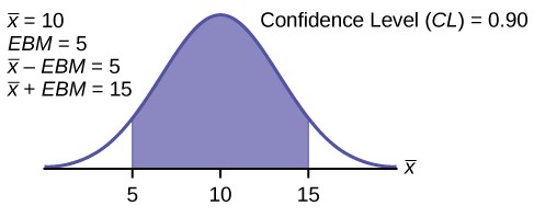
A confidence interval for a population mean with a known standard deviation is based on the fact that the sampling distribution of the sample means follow an approximately normal distribution. Suppose that our sample has a mean of x– =
10, and we have constructed the 90% confidence interval (5, 15) where EBM = 5.
To get a 90% confidence interval, we must include the central 90% of the probability of the normal distribution. If we include the central 90%, we leave out a total of α = 10% in both tails, or 5% in each tail, of the normal distribution.
Figure 8.3
This is a normal distribution curve. The peak of the curve coincides with the point 10 on the horizontal axis. The points 5 and 15 are labeled on the axis. Vertical lines are drawn from these points to the curve, and the region between the lines is shaded. The shaded region has area equal to 0.90.
To capture the central 90%, we must go out 1.645 standard deviations on either side of the calculated sample mean. The value 1.645 is the z-score from a standard normal probability distribution that puts an area of 0.90 in the center, an area of
- in the far left tail, and an area of 0.05 in the far right tail.
It is important that the standard deviation used must be appropriate for the parameter we are estimating, so in this section we need to use the standard deviation that applies to the sampling distribution for means which we studied with the Central
n
Limit Theorem and is, σ .
Calculating the Confidence Interval Using EMB
To construct a confidence interval estimate for an unknown population mean, we need data from a random sample. The steps to construct and interpret the confidence interval are:
- Calculate the sample mean x– from the sample data. Remember, in this section we know the population standard
deviation σ.
- Find the z-score from the standard normal table that corresponds to the confidence level desired.
- Calculate the error bound EBM.
- Construct the confidence interval.
- Write a sentence that interprets the estimate in the context of the situation in the problem.
We will first examine each step in more detail, and then illustrate the process with some examples.
Finding the z-score for the Stated Confidence Level
When we know the population standard deviation σ, we use a standard normal distribution to calculate the error bound EBM and construct the confidence interval. We need to find the value of z that puts an area equal to the confidence level (in decimal form) in the middle of the standard normal distribution Z ~ N(0, 1).
The confidence level, CL, is the area in the middle of the standard normal distribution. CL = 1 – α, so α is the area that is split equally between the two tails. Each of the tails contains an area equal to α .
2
The z-score that has an area to the right of α
2
is denoted by Zα .
2
For example, when CL = 0.95, α = 0.05 and α
2
= 0.025; we write Zα
2
= Z0.025 .
The area to the right of Z0.025 is 0.025 and the area to the left of Z0.025 is 1 – 0.025 = 0.975.
2
Zα = Z0.025 = 1.96 , using a standard normal probability table. We will see later that we can use a different probability
table, the Student’s t-distribution, for finding the number of standard deviations of commonly used levels of confidence.
Calculating the Error Bound (EBM)
⎛⎞⎛ σ ⎞
The error bound formula for an unknown population mean μ when the population standard deviation σ is known is
- EBM = Zα
⎝ 2 ⎠⎝ n⎠
Constructing the Confidence Interval––
- Theconfidenceintervalestimatehastheformat( x – EBM, x + EBM)ortheformula:
- − Z
⎛ σ ⎞ ≤ µ ≤ X– + Z
⎛ σ ⎞
α⎝ n⎠α⎝ n⎠
The graph gives a picture of the entire situation.
CL + α + α
22
= CL + α = 1.
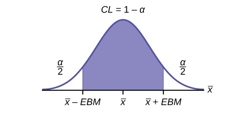
Figure 8.4
Example 8.1Suppose we are interested in the mean scores on an exam. A random sample of 36 scores is taken and gives asample mean (sample mean score) of 68 ( X- = 68). In this example we have the unusual knowledge that the population standard deviation is 3 points. Do not count on knowing the population parameters outside of textbook examples. Find a confidence interval estimate for the population mean exam score (the mean score on all exams).Find a 90% confidence interval for the true (population) mean of statistics exam scores.Solution 8.1The solution is shown step-by-step.To find the confidence interval, you need the sample mean,, and the EBM.x-x-= 68EBM =⎛⎝Zα⎠ ⎝⎞ ⎛ σ ⎞2n⎠σ = 3; n = 36; The confidence level is 90% (CL = 0.90)CL = 0.90 so α = 1 – CL = 1 – 0.90 = 0.10α2= 0.05Zα = z0.052The area to the right of Z0.05 is 0.05 and the area to the left of Z0.05 is 1 – 0.05 = 0.95.
This OpenStax book is available for free at http://cnx.org/content/col11776/1.33
2
Zα = Z0.05 = 1.645
⎠
This can be found using a computer, or using a probability table for the standard normal distribution. Because the common levels of confidence in the social sciences are 90%, 95% and 99% it will not be long until you become familiar with the numbers , 1.645, 1.96, and 2.56
⎛
EBM = (1.645) ⎝
3 ⎞ = 0.8225
36
x– – EBM = 68 – 0.8225 = 67.1775
x– + EBM = 68 + 0.8225 = 68.8225
The 90% confidence interval is (67.1775, 68.8225). Interpretation
We estimate with 90% confidence that the true population mean exam score for all statistics students is between
67.18 and 68.82.
Example 8.2Suppose we change the original problem in Example 8.1 by using a 95% confidence level. Find a 95% confidence interval for the true (population) mean statistics exam score.Solution 8.2Figure 8.5µ = x_ ± Zα⎝⎛ σ ⎞n⎠
⎝
µ = 68 ± 1.96⎛
⎞
3
36⎠
67.02 ≤ µ ≤ 68.98
σ = 3; n = 36; The confidence level is 95% (CL = 0.95).
CL = 0.95 so α = 1 – CL = 1 – 0.95 = 0.05
2
Zα = Z0.025 = 1.96
Notice that the EBM is larger for a 95% confidence level in the original problem.
Comparing the results
The 90% confidence interval is (67.18, 68.82). The 95% confidence interval is (67.02, 68.98). The 95% confidence interval is wider. If you look at the graphs, because the area 0.95 is larger than the area 0.90, it makes sense that the 95% confidence interval is wider. To be more confident that the confidence interval actually does contain the true value of the population mean for all statistics exam scores, the confidence interval necessarily needs to be wider. This demonstrates a very important principle of confidence intervals. There is a trade off between the level of confidence and the width of the interval. Our desire is to have a narrow confidence interval, huge wide intervals provide little information that is useful. But we would also like to have a high level of confidence in our interval. This demonstrates that we cannot have both.
Figure 8.6
Summary: Effect of Changing the Confidence Level
- Increasing the confidence level makes the confidence interval wider.
- Decreasing the confidence level makes the confidence interval narrower.
And again here is the formula for a confidence interval for an unknown mean assuming we have the population standard deviation:
X– − Z
⎛ σ ⎞ ≤ µ ≤ X– + Z
⎛ σ ⎞
α⎝ n⎠α⎝ n⎠
n
The standard deviation of the sampling distribution was provided by the Central Limit Theorem as σ
. While
we infrequently get to choose the sample size it plays an important role in the confidence interval. Because the sample size is in the denominator of the equation, as n increases it causes the standard deviation of the sampling distribution to idecrease and thus the width of the confidence interval to decrease. We have met this before as we reviewed the effects of sample size on the Central Limit Theorem. There we saw that as n increases the sampling distribution narrows until in the limit it collapses on the true population mean.
Example 8.3Suppose we change the original problem in Example 8.1 to see what happens to the confidence interval if the
This OpenStax book is available for free at http://cnx.org/content/col11776/1.33
sample size is changed.
Leave everything the same except the sample size. Use the original 90% confidence level. What happens to the confidence interval if we increase the sample size and use n = 100 instead of n = 36? What happens if we decrease the sample size to n = 25 instead of n = 36?
Solution 8.3
Solution A
µ = x_ ± Z
⎛ σ ⎞
α⎝ n⎠
⎝
µ = 68 ± 1.645⎛
3 ⎞ 100
⎠
67.5065 ≤ µ ≤ 68.4935
If we increase the sample size n to 100, we decrease the width of the confidence interval relative to the original sample size of 36 observations.
Solution 8.3
Solution B
µ = x_ ± Z
⎛ σ ⎞
α⎝ n⎠
⎝
µ = 68 ± 1.645⎛
⎞
3
25⎠
67.013 ≤ µ ≤ 68.987
If we decrease the sample size n to 25, we increase the width of the confidence interval by comparison to the original sample size of 36 observations.
Summary: Effect of Changing the Sample Size
- Increasing the sample size makes the confidence interval narrower.
- Decreasing the sample size makes the confidence interval wider.
We have already seen this effect when we reviewed the effects of changing the size of the sample, n, on the Central Limit Theorem. See Figure 7.7 to see this effect. Before we saw that as the sample size increased the standard deviation of the sampling distribution decreases. This was why we choose the sample mean from a large sample as compared to a small sample, all other things held constant.
Thus far we assumed that we knew the population standard deviation. This will virtually never be the case. We will have the sample standard deviation, s, however. This is a point estimate for the population standard deviation and can be substituted into the formula for confidence intervals for a mean under certain circumstances. We just saw the effect the sample size has on the width of confidence interval and the impact on the sampling distribution for our discussion of the Central Limit Theorem. We can invoke this to substitute the point estimate for the standard deviation if the sample size is large “enough”. Simulation studies indicate that 30 observations or more will be sufficient to eliminate any meaningful bias in the estimated confidence interval.
Example 8.4Spring break can be a very expensive holiday. A sample of 80 students is surveyed, and the average amount spent by students on travel and beverages is $593.84. The sample standard deviation is approximately $369.34.Construct a 92% confidence interval for the population mean amount of money spent by spring breakers.
Solution 8.4
We begin with the confidence interval for a mean. We use the formula for a mean because the random variable is dollars spent and this is a continuous random variable. The point estimate for the population standard deviation, s, has been substituted for the true population standard deviation because with 80 observations there is no concern for bias in the estimate of the confidence interval.
µ = x¯ ± ⎡Z(a /2) s ⎤
⎣n⎦
Substituting the values into the formula, we have:
µ = 593.84 ± ⎡1.75369.34⎤
⎣80 ⎦
Z(a / 2) is found on the standard normal table by looking up 0.46 in the body of the table and finding the number of standard deviations on the side and top of the table; 1.75. The solution for the interval is thus:
µ = 593.84 ± 72.2636 = ⎛521.57, 666.10⎞
⎝⎠
$ 521.58 ≤ µ ≤ $ 666.10
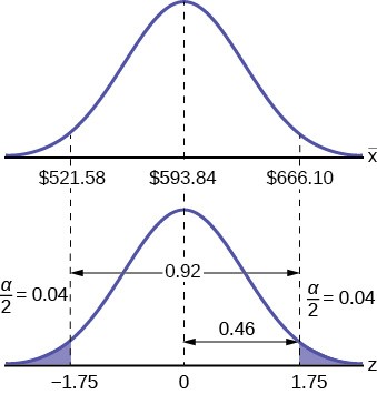
Figure 8.7
Formula Review
The general form for a confidence interval for a single population mean, known standard deviation, normal distribution is
given by X– − Z ⎛ σ ⎞ ≤ µ ≤ X– + Z ⎛ σ ⎞ This formula is used when the population standard deviation is known.
α⎝ n⎠α⎝ n⎠
CL = confidence level, or the proportion of confidence intervals created that are expected to contain the true population parameter
α = 1 – CL = the proportion of confidence intervals that will not contain the population parameter
z α = the z-score with the property that the area to the right of the z-score is∝
this is the z-score used in the calculation
22
This OpenStax book is available for free at http://cnx.org/content/col11776/1.33
of “EBM where α = 1 – CL.
| A Confidence Interval for a Population Standard Deviation Unknown, Small Sample Case
In practice, we rarely know the population standard deviation. In the past, when the sample size was large, this did not present a problem to statisticians. They used the sample standard deviation s as an estimate for σ and proceeded as before to calculate a confidence interval with close enough results. This is what we did in Example 8.4 above. The point estimate for the standard deviation, s, was substituted in the formula for the confidence interval for the population standard deviation. In this case there 80 observation well above the suggested 30 observations to eliminate any bias from a small sample. However, statisticians ran into problems when the sample size was small. A small sample size caused inaccuracies in the confidence interval.
William S. Goset (1876–1937) of the Guinness brewery in Dublin, Ireland ran into this problem. His experiments with hops and barley produced very few samples. Just replacing σ with s did not produce accurate results when he tried to calculate a confidence interval. He realized that he could not use a normal distribution for the calculation; he found that the actual distribution depends on the sample size. This problem led him to “discover” what is called the Student’s t-distribution. The name comes from the fact that Gosset wrote under the pen name “A Student.”
If you draw a simple random sample of size n from a population with mean μ and unknown population standard deviation
- ⎛ s ⎞
and calculate the t-score t = x– – µ , then the t-scores follow a Student’s t-distribution with n – 1 degrees of freedom.
⎝ n⎠
μ. For each sample size n, there is a different Student’s t-distribution.
(x – x– values) to calculate s. Because the sum of the deviations is zero, we can find the last deviation once we know the
other n – 1 deviations. The other n – 1 deviations can change or vary freely. We call the number n – 1 the degrees of freedom (df) in recognition that one is lost in the calculations. The effect of losing a degree of freedom is that the t-value increases and the confidence interval increases in width.
Properties of the Student’s t-Distribution
- The graph for the Student’s t-distribution is similar to the standard normal curve and at infinite degrees of freedom it is the normal distribution. You can confirm this by reading the bottom line at infinite degrees of freedom for a familiar level of confidence, e.g. at column 0.05, 95% level of confidence, we find the t-value of 1.96 at infinite degrees of freedom.
- The mean for the Student’s t-distribution is zero and the distribution is symmetric about zero, again like the standard normal distribution.
- The Student’s t-distribution has more probability in its tails than the standard normal distribution because the spread of the t-distribution is greater than the spread of the standard normal. So the graph of the Student’s t-distribution will be thicker in the tails and shorter in the center than the graph of the standard normal distribution.
- The exact shape of the Student’s t-distribution depends on the degrees of freedom. As the degrees of freedom increases, the graph of Student’s t-distribution becomes more like the graph of the standard normal distribution.
- The underlying population of individual observations is assumed to be normally distributed with unknown population mean μ and unknown population standard deviation σ. This assumption comes from the Central Limit theorem because the individual observations in this case are the x¯ s of the sampling distribution. The size of the underlying population is generally not relevant unless it is very small. If it is normal then the assumption is met and doesn’t need discussion.
A probability table for the Student’s t-distribution is used to calculate t-values at various commonly-used levels of confidence. The table gives t-scores that correspond to the confidence level (column) and degrees of freedom (row). When using a t-table, note that some tables are formatted to show the confidence level in the column headings, while the column headings in some tables may show only corresponding area in one or both tails. Notice that at the bottom the table will show the t-value for infinite degrees of freedom. Mathematically, as the degrees of freedom increase, the t distribution approaches the standard normal distribution. You can find familiar Z-values by looking in the relevant alpha column and reading value
in the last row.
A Student’s t table (See Appendix A) gives t-scores given the degrees of freedom and the right-tailed probability.
The Student’s t distribution has one of the most desirable properties of the normal: it is symmetrical. What the Student’s t distribution does is spread out the horizontal axis so it takes a larger number of standard deviations to capture the same amount of probability. In reality there are an infinite number of Student’s t distributions, one for each adjustment to the sample size. As the sample size increases, the Student’s t distribution become more and more like the normal distribution. When the sample size reaches 30 the normal distribution is usually substituted for the Student’s t because they are so much alike. This relationship between the Student’s t distribution and the normal distribution is shown in Figure 8.8.
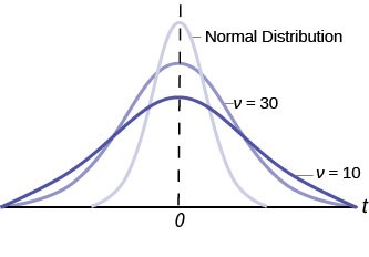
This is another example of one distribution limiting another one, in this case the normal distribution is the limiting distribution of the Student’s t when the degrees of freedom in the Student’s t approaches infinity. This conclusion comes directly from the derivation of the Student’s t distribution by Mr. Gosset. He recognized the problem as having few observations and no estimate of the population standard deviation. He was substituting the sample standard deviation and getting volatile results. He therefore created the Student’s t distribution as a ratio of the normal distribution and Chi squared distribution. The Chi squared distribution is itself a ratio of two variances, in this case the sample variance and the unknown population variance. The Student’s t distribution thus is tied to the normal distribution, but has degrees of freedom that come from those of the Chi squared distribution. The algebraic solution demonstrates this result.
zχ 2 v
Development of Student’s t-distribution:
- t =
Where Z is the standard normal distribution and χ2 is the chi-squared distribution with v degrees of freedom.
σ s2(n − 1)σ 2(n − 1)
⎝⎠
⎛ x¯ − µ⎞
- t =
by substitution, and thus Student’s t with v = n − 1 degrees of freedom is:
s
3. t = x¯ − µ
n
Restating the formula for a confidence interval for the mean for cases when the sample size is smaller than 30 and we do not know the population standard deviation, σ:
x– – t
⎛ s ⎞ ≤ µ ≤ x– + t
⎛ s ⎞
v,α⎝ n⎠v,α⎝ n⎠
This OpenStax book is available for free at http://cnx.org/content/col11776/1.33
Here the point estimate of the population standard deviation, s has been substituted for the population standard deviation, σ, and tν,α has been substituted for Zα. The Greek letter ν (pronounced nu) is placed in the general formula in recognition that there are many Student tv distributions, one for each sample size. ν is the symbol for the degrees of freedom of the distribution and depends on the size of the sample. Often df is used to abbreviate degrees of freedom. For this type of problem, the degrees of freedom is ν = n-1, where n is the sample size. To look up a probability in the Student’s t table we have to know the degrees of freedom in the problem.
Example 8.5
The average earnings per share (EPS) for 10 industrial stocks randomly selected from those listed on the Dow- Jones Industrial Average was found to be X– = 1.85 with a standard deviation of s=0.395. Calculate a 99%
confidence interval for the average EPS of all the industrials listed on the DJIA.
x– – t
⎛ s ⎞ ≤ µ ≤ x– + t
⎛ s ⎞
v,α⎝ n⎠v,α⎝ n⎠
Solution 8.5
To help visualize the process of calculating a confident interval we draw the appropriate distribution for the problem. In this case this is the Student’s t because we do not know the population standard deviation and the sample is small, less than 30.
Figure 8.9
To find the appropriate t-value requires two pieces of information, the level of confidence desired and the degrees of freedom. The question asked for a 99% confidence level. On the graph this is shown where (1-α) , the level of confidence , is in the unshaded area. The tails, thus, have .005 probability each, α/2. The degrees of freedom for this type of problem is n-1= 9. From the Student’s t table, at the row marked 9 and column marked .005, is the number of standard deviations to capture 99% of the probability, 3.2498. These are then placed on the graph remembering that the Student’s t is symmetrical and so the t-value is both plus or minus on each side of the mean.
Inserting these values into the formula gives the result. These values can be placed on the graph to see the relationship between the distribution of the sample means, X– ‘s and the Student’s t distribution.
µ = X– ± tα/2,df=n-1 s = 1.851 ± 3.24980.395 = 1.8551 ± 0.406
We state the formal conclusion as :
n10
1.445 ≤ µ ≤ 2.257
With 99% confidence level, the average EPS of all the industries listed at DJIA is from $1.44 to $2.26.
8.5 You do a study of hypnotherapy to determine how effective it is in increasing the number of hours of sleep subjects get each night. You measure hours of sleep for 12 subjects with the following results. Construct a 95% confidence interval for the mean number of hours slept for the population (assumed normal) from which you took the data.8.2; 9.1; 7.7; 8.6; 6.9; 11.2; 10.1; 9.9; 8.9; 9.2; 7.5; 10.5
| A Confidence Interval for A Population Proportion
Investors in the stock market are interested in the true proportion of stocks that go up and down each week. Businesses that sell personal computers are interested in the proportion of households in the United States that own personal computers. Confidence intervals can be calculated for the true proportion of stocks that go up or down each week and for the true proportion of households in the United States that own personal computers.
The procedure to find the confidence interval for a population proportion is similar to that for the population mean, but the formulas are a bit different although conceptually identical. While the formulas are different, they are based upon the same mathematical foundation given to us by the Central Limit Theorem. Because of this we will see the same basic format using the same three pieces of information: the sample value of the parameter in question, the standard deviation of the relevant sampling distribution, and the number of standard deviations we need to have the confidence in our estimate that we desire.
How do you know you are dealing with a proportion problem? First, the underlying distribution has a binary random variable and therefore is a binomial distribution. (There is no mention of a mean or average.) If X is a binomial random variable, then X ~ B(n, p) where n is the number of trials and p is the probability of a success. To form a sample proportion, take X, the random variable for the number of successes and divide it by n, the number of trials (or the sample size). The random variable P′ (read “P prime”) is the sample proportion,
n
P′ = X
(Sometimes the random variable is denoted as P^ , read “P hat”.)
p′ = the estimated proportion of successes or sample proportion of successes (p′ is a point estimate for p, the true population proportion, and thus q is the probability of a failure in any one trial.)
x = the number of successes in the sample
n = the size of the sample
The formula for the confidence interval for a population proportion follows the same format as that for an estimate of a population mean. Remembering the sampling distribution for the proportion from Chapter 7, the standard deviation was found to be:
This OpenStax book is available for free at http://cnx.org/content/col11776/1.33
p⎛1 − p⎞⎝⎠n
σp’ =
The confidence interval for a population proportion, therefore, becomes:
p = p′ ± ⎡Z⎛ ⎞
p′⎛1 − p′⎞⎤
2
⎣ ⎝a⎠
⎝ n⎠⎦
Z a
⎛ ⎞
⎝2⎠
is set according to our desired degree of confidence and
is the standard deviation of the sampling
p′⎛1 − p′⎞⎝⎠n
distribution.
The sample proportions p′ and q′ are estimates of the unknown population proportions p and q. The estimated proportions p′ and q′ are used because p and q are not known.
Remember that as p moves further from 0.5 the binomial distribution becomes less symmetrical. Because we are estimating the binomial with the symmetrical normal distribution the further away from symmetrical the binomial becomes the less confidence we have in the estimate.
This conclusion can be demonstrated through the following analysis. Proportions are based upon the binomial probability distribution. The possible outcomes are binary, either “success” or “failure”. This gives rise to a proportion, meaning the percentage of the outcomes that are “successes”. It was shown that the binomial distribution could be fully understood if we knew only the probability of a success in any one trial, called p. The mean and the standard deviation of the binomial were found to be:
µ = np
σ = npq
It was also shown that the binomial could be estimated by the normal distribution if BOTH np AND nq were greater than 5. From the discussion above, it was found that the standardizing formula for the binomial distribution is:
Z =
p’ – p
⎛ pq⎞
⎝ n ⎠
which is nothing more than a restatement of the general standardizing formula with appropriate substitutions for μ and σ from the binomial. We can use the standard normal distribution, the reason Z is in the equation, because the normal distribution is the limiting distribution of the binomial. This is another example of the Central Limit Theorem. We have already seen that the sampling distribution of means is normally distributed. Recall the extended discussion in Chapter 7 concerning the sampling distribution of proportions and the conclusions of the Central Limit Theorem.
We can now manipulate this formula in just the same way we did for finding the confidence intervals for a mean, but to find the confidence interval for the binomial population parameter, p.
p’q’n
p’q’n
p’ – Zα≤ p ≤ p’ + Zα
Where p′ = x/n, the point estimate of p taken from the sample. Notice that p′ has replaced p in the formula. This is because we do not know p, indeed, this is just what we are trying to estimate.
Unfortunately, there is no correction factor for cases where the sample size is small so np′ and nq’ must always be greater than 5 to develop an interval estimate for p.
Example 8.6Suppose that a market research firm is hired to estimate the percent of adults living in a large city who have cell phones. Five hundred randomly selected adult residents in this city are surveyed to determine whether they have cell phones. Of the 500 people sampled, 421 responded yes – they own cell phones. Using a 95% confidence level, compute a confidence interval estimate for the true proportion of adult residents of this city who have cell phones.Solution 8.6The solution step-by-step.
Let X = the number of people in the sample who have cell phones. X is binomial: the random variable is binary, people either have a cell phone or they do not.
To calculate the confidence interval, we must find p′, q′. n = 500
x = the number of successes in the sample = 421
p′ = x = 421 = 0.842
n500
p′ = 0.842 is the sample proportion; this is the point estimate of the population proportion.
q′ = 1 – p′ = 1 – 0.842 = 0.158
⎝ ⎠
Since the requested confidence level is CL = 0.95, then α = 1 – CL = 1 – 0.95 = 0.05 ⎛α⎞ = 0.025.
2
2
Then z α = z0.025 = 1.96
This can be found using the Standard Normal probability table in Appendix A. This can also be found in the students t table at the 0.025 column and infinity degrees of freedom because at infinite degrees of freedom the students t distribution becomes the standard normal distribution, Z.
The confidence interval for the true binomial population proportion is
p’q’n
p’q’n
p’ – Zα≤ p ≤ p’ + Zα
Substituting in the values from above we find he confidence inte val is : 0.810 ≤ p ≤ 0.874
Interpretation
We estimate with 95% confidence that between 81% and 87.4% of all adult residents of this city have cell phones.
Explanation of 95% Confidence Level
Ninety-five percent of the confidence intervals constructed in this way would contain the true value for the population proportion of all adult residents of this city who have cell phones.
8.6 Suppose 250 randomly selected people are surveyed to determine if they own a tablet. Of the 250 surveyed, 98 reported owning a tablet. Using a 95% confidence level, compute a confidence interval estimate for the true proportion of people who own tablets.
Example 8.7The Dundee Dog Training School has a larger than average proportion of clients who compete in competitive professional events. A confidence interval for the population proportion of dogs that compete in professional events from 150 different training schools is constructed. The lower limit is determined to be 0.08 and the upper limit is determined to be 0.16. Determine the level of confidence used to construct the interval of the population proportion of dogs that compete in professional events.Solution 8.7We begin with the formula for a confidence interval for a proportion because the random variable is binary; either
This OpenStax book is available for free at http://cnx.org/content/col11776/1.33
the client competes in professional competitive dog events or they don’t.
2
p = p′ ± ⎡Z⎛ ⎞
p′⎛1 − p′⎞⎤
Next we find the sample proportion:
⎣ ⎝a⎠
⎝ n⎠⎦
2
p′ = 0.08 + 0.16 = 0.12
The ± that makes up the confidence interval is thus 0.04; 0.12 + 0.04 = 0.16 and 0.12 − 0.04 = 0.08, the boundaries of the confidence interval. Finally, we solve for Z.
⎡Z ⋅ 0.12(1 − 0.12)⎤ = 0.04 , therefore Z = 1.51
⎣150⎦
And then look up the probability for 1.51 standard deviations on the standard normal table.
⎝
⎠
⎝
⎠
p⎛Z = 1.51⎞ = 0.4345 , p⎛Z⎞ ⋅ 2 = 0.8690 or 86.90 % .
Example 8.8
A financial officer for a company wants to estimate the percent of accounts receivable that are more than 30 days overdue. He surveys 500 accounts and finds that 300 are more than 30 days overdue. Compute a 90% confidence interval for the true percent of accounts receivable that are more than 30 days overdue, and interpret the confidence interval.
Solution 8.8
- The solution is step-by-step:
x = 300 and n = 500
p′ = x = 300 = 0.600
n500
q′ = 1 – p′ = 1 – 0.600 = 0.400
⎝ ⎠
Since confidence level = 0.90, then α = 1 – confidence level = (1 – 0.90) = 0.10 ⎛α⎞ = 0.05
2
Zα = Z0.05 = 1.645
2
This Z-value can be found using a standard normal probability table. The student’s t-table can also be used by entering the table at the 0.05 column and reading at the line for infinite degrees of freedom. The t-distribution is the normal distribution at infinite degrees of freedom. This is a handy trick to remember in finding Z-values for commonly used levels of confidence. We use this formula for a confidence interval for a proportion:
p’ – Zα p’q’ ≤ p ≤ p’ + Zα p’q’
nn
Substituting in the values from above we find the confidence interval for the true binomial population proportion is 0.564 ≤ p ≤ 0.636
Interpretation
- We estimate with 90% confidence that the true percent of all accounts receivable overdue 30 days is between 56.4% and 63.6%.
- Alternate Wording: We estimate with 90% confidence that between 56.4% and 63.6% of ALL accounts are overdue 30 days.
Explanation of 90% Confidence Level
Ninety percent of all confidence intervals constructed in this way contain the true value for the population percent of accounts receivable that are overdue 30 days.
8.8 A student polls his school to see if students in the school district are for or against the new legislation regarding school uniforms. She surveys 600 students and finds that 480 are against the new legislation.Compute a 90% confidence interval for the true percent of students who are against the new legislation, and interpret the confidence interval.In a sample of 300 students, 68% said they own an iPod and a smart phone. Compute a 97% confidence interval for the true percent of students who own an iPod and a smartphone.
| Calculating the Sample Size n: Continuous and Binary Random Variables
Continuous Random Variables
Usually we have no control over the sample size of a data set. However, if we are able to set the sample size, as in cases where we are taking a survey, it is very helpful to know just how large it should be to provide the most information. Sampling can be very costly in both time and product. Simple telephone surveys will cost approximately $30.00 each, for example, and some sampling requires the destruction of the product.
If we go back to our standardizing formula for the sampling distribution for means, we can see that it is possible to solve it
for n. If we do this we have ⎛ X– – µ⎞ in the denominator.
⎝⎠
n = Zα2 σ 2
⎛ X– – µ⎞2
Zα2 σ 2
=
e2
⎝⎠
Because we have not taken a sample yet we do not know any of the variables in the formula except that we can set Zα to the level of confidence we desire just as we did when determining confidence intervals. If we set a predetermined acceptable
error, or tolerance, for the difference between X– and μ, called e in the formula, we are much further in solving for the
sample size n. We still do not know the population standard deviation, σ. In practice, a pre-survey is usually done which allows for fine tuning the questionnaire and will give a sample standard deviation that can be used. In other cases, previous information from other surveys may be used for σ in the formula. While crude, this method of determining the sample size may help in reducing cost significantly. It will be the actual data gathered that determines the inferences about the population, so caution in the sample size is appropriate calling for high levels of confidence and small sampling errors.
Binary Random Variables
What was done in cases when looking for the mean of a distribution can also be done when sampling to determine the population parameter p for proportions. Manipulation of the standardizing formula for proportions gives:
2
n = Zα2 pq
e
where e = (p′-p), and is the acceptable sampling error, or tolerance, for this application. This will be measured in percentage points.
In this case the very object of our search is in the formula, p, and of course q because q =1-p. This result occurs because the binomial distribution is a one parameter distribution. If we know p then we know the mean and the standard deviation. Therefore, p shows up in the standard deviation of the sampling distribution which is where we got this formula. If, in an
This OpenStax book is available for free at http://cnx.org/content/col11776/1.33
abundance of caution, we substitute 0.5 for p we will draw the largest required sample size that will provide the level of confidence specified by Zα and the tolerance we have selected. This is true because of all combinations of two fractions that add to one, the largest multiple is when each is 0.5. Without any other information concerning the population parameter p, this is the common practice. This may result in oversampling, but certainly not under sampling, thus, this is a cautious approach.
There is an interesting trade-off between the level of confidence and the sample size that shows up here when considering the cost of sampling. Table 8.1 shows the appropriate sample size at different levels of confidence and different level of the acceptable error, or tolerance.
|
Required Sample Size (95%) |
Tolerance Level |
|
|
1691 |
2401 |
2% |
|
752 |
1067 |
3% |
|
271 |
384 |
5% |
|
68 |
96 |
10% |
Table 8.1
This table is designed to show the maximum sample size required at different levels of confidence given an assumed p= 0.5 and q=0.5 as discussed above.
The acceptable error, called tolerance in the table, is measured in plus or minus values from the actual proportion. For example, an acceptable error of 5% means that if the sample proportion was found to be 26 percent, the conclusion would be that the actual population proportion is between 21 and 31 percent with a 90 percent level of confidence if a sample of 271 had been taken. Likewise, if the acceptable error was set at 2%, then the population proportion would be between 24 and 28 percent with a 90 percent level of confidence, but would require that the sample size be increased from 271 to 1,691. If we wished a higher level of confidence, we would require a larger sample size. Moving from a 90 percent level of confidence to a 95 percent level at a plus or minus 5% tolerance requires changing the sample size from 271 to 384. A very common sample size often seen reported in political surveys is 384. With the survey results it is frequently stated that the results are good to a plus or minus 5% level of “accuracy”.
Example 8.9Suppose a mobile phone company wants to determine the current percentage of customers aged 50+ who use text messaging on their cell phones. How many customers aged 50+ should the company survey in order to be 90% confident that the estimated (sample) proportion is within three percentage points of the true population proportion of customers aged 50+ who use text messaging on their cell phones.Solution 8.9From the problem, we know that the acceptable error, e, is 0.03 (3%=0.03) and z α z0.05 = 1.645 because the2confidence level is 90%. The acceptable error, e, is the difference between the actual population proportion p, and the sample proportion we expect to get from the sample.However, in order to find n, we need to know the estimated (sample) proportion p′. Remember that q′ = 1 – p′. But, we do not know p′ yet. Since we multiply p′ and q′ together, we make them both equal to 0.5 because p′q′ = (0.5)(0.5) = 0.25 results in the largest possible product. (Try other products: (0.6)(0.4) = 0.24; (0.3)(0.7)= 0.21; (0.2)(0.8) = 0.16 and so on). The largest possible product gives us the largest n. This gives us a large enough sample so that we can be 90% confident that we are within three percentage points of the true population proportion. To calculate the sample size n, use the formula and make the substitutions.n = z2 p′ q′e2givesn = 1.6452(0.5)(0.5) = 751.70.032Round the answer to the next higher value. The sample size should be 752 cell phone customers aged 50+ in order
to be 90% confident that the estimated (sample) proportion is within three percentage points of the true population proportion of all customers aged 50+ who use text messaging on their cell phones.
8.9 Suppose an internet marketing company wants to determine the current percentage of customers who click on ads on their smartphones. How many customers should the company survey in order to be 90% confident that the estimated proportion is within five percentage points of the true population proportion of customers who click on ads on their smartphones?
This OpenStax book is available for free at http://cnx.org/content/col11776/1.33
binomial RV X is defined as the number of successes in n trials. The notation is: X~B(n,p). The mean is μ = np and
the standard deviation is σ = npq . The probability of exactly x successes in n trials is P⎛X = x⎞ = ⎛n⎞
px qn − x
⎝⎠⎝x⎠
.
Confidence Interval (CI) an interval estimate for an unknown population parameter. This depends on:
- the desired confidence level,
- information that is known about the distribution (for example, known standard deviation),
- the sample and its size.
Degrees of Freedom (df) the number of objects in a sample that are free to vary
1 – (x – µ)2 / 2σ 2
Normal Distribution
a continuous random variable (RV) with pdf f (x) = e, where μ is the mean
σ 2π
of the distribution and σ is the standard deviation, notation: X ~ N(μ,σ). If μ = 0 and σ = 1, the RV is called the standard normal distribution.
Parameter a numerical characteristic of a population
Point Estimate a single number computed from a sample and used to estimate a population parameter
- It is continuous and assumes any real values.
- The pdf is symmetrical about its mean of zero.
- It approaches the standard normal distribution as n get larger.
- There is a “family of t–distributions: each representative of the family is completely defined by the number of degrees of freedom, which depends upon the application for which the t is being used.
CHAPTER REVIEW
A Confidence Interval for a Population Standard Deviation Unknown, Small Sample Case
In many cases, the researcher does not know the population standard deviation, σ, of the measure being studied. In these
cases, it is common to use the sample standard deviation, s, as an estimate of σ. The normal distribution creates accurate confidence intervals when σ is known, but it is not as accurate when s is used as an estimate. In this case, the Student’s t-distribution is much better. Define a t-score using the following formula:
t =
x– – µ
s n
The t-score follows the Student’s ⎛t-di⎞stribution with n – 1 degrees of freedom. The confidence interval under this
distribution is calculated with x– ± ⎝t α⎠ s where t α is the t-score with area to the right equal to α , s is the sample
2n22
standard deviation, and n is the sample size. Use a table, calculator, or computer to find t α
2
for a given α.
A Confidence Interval for A Population Proportion
Some statistical measures, like many survey questions, measure qualitative rather than quantitative data. In this case, the population parameter being estimated is a proportion. It is possible to create a confidence interval for the true population proportion following procedures similar to those used in creating confidence intervals for population means. The formulas are slightly different, but they follow the same reasoning.
Let p′ represent the sample proportion, x/n, where x represents the number of successes and n represents the sample size. Let q′ = 1 – p′. Then the confidence interval for a population proportion is given by the following formula:
p’q’n
p’q’n
p’ – Zα≤ p ≤ p’ + Zα
Calculating the Sample Size n: Continuous and Binary Random Variables
Sometimes researchers know in advance that they want to estimate a population mean within a specific margin of error for a given level of confidence. In that case, solve the relevant confidence interval formula for n to discover the size of the sample that is needed to achieve this goal:
n =
Zα2 σ 2
⎝
⎠
⎛ x– – µ⎞2
If the random variable is binary then the formula for the appropriate sample size to maintain a particular level of confidence with a specific tolerance level is given by
2
n = Zα2 pq
e
FORMULA REVIEW
The general form for a confidence interval for a single mean, population standard deviation unknown, and sample size less than 30 Student’s t is given by:
– t
⎛ s ⎞ ≤ µ ≤ x– + t
⎛ s ⎞
s = the standard deviation of sample values.
v,α⎝ n⎠
v,α⎝ n⎠
s
t =x– − µ is the formula for the t-score which measures
n
n
A Confidence Interval for A Population Proportion
how far away a measure is from the population mean in the Student’s t-distribution
p′= x
where x represents the number of successes in a
df = n – 1; the degrees of freedom for a Student’s t- distribution where n represents the size of the sample
T~tdf the random variable, T, has a Student’s t-distribution with df degrees of freedom
sample and n represents the sample size. The variable p′ is
the sample proportion and serves as the point estimate for the true population proportion.
q′ = 1 – p′
This OpenStax book is available for free at http://cnx.org/content/col11776/1.33
The variable p′ has a binomial distribution that can be approximated with the normal distribution shown here. The confidence interval for the true population proportion is given by the formula:
Calculating the Sample Size n: Continuous and Binary Random Variables
Z 2 σ 2
p’ – Zα
n =
≤ p ≤ p’ + Zα Zα 2 p′ q′
p’q’n
p’q’n
2provides the number of observations
e2
n = ⎛⎝ x– – µ⎞⎠2 = the formula used to determine the sample size (n) needed to achieve a desired margin of error at a given level of confidence for a continuous random variable
2
Z 2 pq
needed to sample to estimate the population proportion,
p, with confidence 1 – α and margin of error e. Where e
= the acceptable difference between the actual population proportion and the sample proportion.
PRACTICE
n = α= the formula used to determine the sample
e
size if the random variable is binary
Use the following information to answer the next five exercises. A hospital is trying to cut down on emergency room wait times. It is interested in the amount of time patients must wait before being called back to be examined. An investigation committee randomly surveyed 70 patients. The sample mean was 1.5 hours with a sample standard deviation of 0.5 hours.
- Identify the following:
- x– =
- sx =
- n =
d. n – 1 =
- Define the random variables X and X– in words.
- Which distribution should you use for this problem?
- Construct a 95% confidence interval for the population mean time spent waiting. State the confidence interval, sketch the graph, and calculate the error bound.
- Explain in complete sentences what the confidence interval means.
Use the following information to answer the next six exercises: One hundred eight Americans were surveyed to determine the number of hours they spend watching television each month. It was revealed that they watched an average of 151 hours each month with a standard deviation of 32 hours. Assume that the underlying population distribution is normal.
- Identify the following:
- x– =
- sx =
- n =
d. n – 1 =
- Define the random variable X in words.
- Define the random variable X– in words.
- Which distribution should you use for this problem?
- Construct a 99% confidence interval for the population mean hours spent watching television per month. (a) State the confidence interval, (b) sketch the graph, and (c) calculate the error bound.
- Why would the error bound change if the confidence level were lowered to 95%?
Use the following information to answer the next 13 exercises: The data in Table 8.2 are the result of a random survey of 39
national flags (with replacement between picks) from various countries. We are interested in finding a confidence interval for the true mean number of colors on a national flag. Let X = the number of colors on a national flag.
|
Freq. |
|
|
1 |
1 |
|
2 |
7 |
|
3 |
18 |
|
4 |
7 |
|
5 |
6 |
Table 8.2
- Calculate the following:
- x– =
- sx =
- n =
- Define the random variable X– in words.
- What is x– estimating?
- Is σx known?
- As a result of your answer to Exercise 8.15, state the exact distribution to use when calculating the confidence interval.
Construct a 95% confidence interval for the true mean number of colors on national flags.
- How much area is in both tails (combined)?
- How much area is in each tail?
- Calculate the following:
- lower limit
- upper limit
- error bound
- The 95% confidence interval is .
- Fill in the blanks on the graph with the areas, the upper and lower limits of the Confidence Interval and the sample mean.
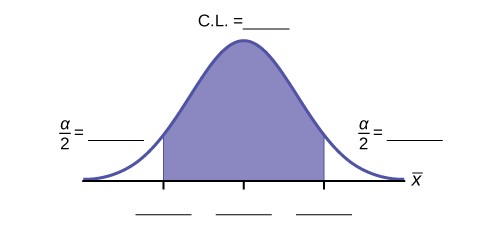
Figure 8.10
This OpenStax book is available for free at http://cnx.org/content/col11776/1.33
- Using the same x– , sx , and level of confidence, suppose that n were 69 instead of 39. Would the error bound become larger or smaller? How do you know?
- Using the same x– , sx , and n = 39, how would the error bound change if the confidence level were reduced to 90%?
Why?
A Confidence Interval for A Population Proportion
Use the following information to answer the next two exercises: Marketing companies are interested in knowing the population percent of women who make the majority of household purchasing decisions.
- When designing a study to determine this population proportion, what is the minimum number you would need to survey to be 90% confident that the population proportion is estimated to within 0.05?
- If it were later determined that it was important to be more than 90% confident and a new survey were commissioned, how would it affect the minimum number you need to survey? Why?
Use the following information to answer the next five exercises: Suppose the marketing company did do a survey. They randomly surveyed 200 households and found that in 120 of them, the woman made the majority of the purchasing decisions. We are interested in the population proportion of households where women make the majority of the purchasing decisions.
- Identify the following:
- x =
- n =
- p′ =
- Define the random variables X and P′ in words.
- Which distribution should you use for this problem?
- Construct a 95% confidence interval for the population proportion of households where the women make the majority of the purchasing decisions. State the confidence interval, sketch the graph, and calculate the error bound.
- List two difficulties the company might have in obtaining random results, if this survey were done by email.
Use the following information to answer the next five exercises: Of 1,050 randomly selected adults, 360 identified themselves as manual laborers, 280 identified themselves as non-manual wage earners, 250 identified themselves as mid- level managers, and 160 identified themselves as executives. In the survey, 82% of manual laborers preferred trucks, 62% of non-manual wage earners preferred trucks, 54% of mid-level managers preferred trucks, and 26% of executives preferred trucks.
- We are interested in finding the 95% confidence interval for the percent of executives who prefer trucks. Define random variables X and P′ in words.
- Which distribution should you use for this problem?
- Construct a 95% confidence interval. State the confidence interval, sketch the graph, and calculate the error bound.
- Suppose we want to lower the sampling error. What is one way to accomplish that?
- The sampling error given in the survey is ±2%. Explain what the ±2% means.
Use the following information to answer the next five exercises: A poll of 1,200 voters asked what the most significant issue was in the upcoming election. Sixty-five percent answered the economy. We are interested in the population proportion of voters who feel the economy is the most important.
- Define the random variable X in words.
- Define the random variable P′ in words.
- Which distribution should you use for this problem?
- Construct a 90% confidence interval, and state the confidence interval and the error bound.
- What would happen to the confidence interval if the level of confidence were 95%?
Use the following information to answer the next 16 exercises: The Ice Chalet offers dozens of different beginning ice- skating classes. All of the class names are put into a bucket. The 5 P.M., Monday night, ages 8 to 12, beginning ice-skating class was picked. In that class were 64 girls and 16 boys. Suppose that we are interested in the true proportion of girls, ages 8 to 12, in all beginning ice-skating classes at the Ice Chalet. Assume that the children in the selected class are a random sample of the population.
- What is being counted?
- In words, define the random variable X.
- Calculate the following:
- x =
- n =
- p′ =
- State the estimated distribution of X. X~
- Define a new random variable P′. What is p′ estimating?
- In words, define the random variable P′.
- State the estimated distribution of P′. Construct a 92% Confidence Interval for the true proportion of girls in the ages 8 to 12 beginning ice-skating classes at the Ice Chalet.
- How much area is in both tails (combined)?
- How much area is in each tail?
- Calculate the following:
- lower limit
- upper limit
- error bound
- The 92% confidence interval is .
- Fill in the blanks on the graph with the areas, upper and lower limits of the confidence interval, and the sample proportion.
Figure 8.11
- In one complete sentence, explain what the interval means.
- Using the same p′ and level of confidence, suppose that n were increased to 100. Would the error bound become larger or smaller? How do you know?
- Using the same p′ and n = 80, how would the error bound change if the confidence level were increased to 98%? Why?
- If you decreased the allowable error bound, why would the minimum sample size increase (keeping the same level of confidence)?
Calculating the Sample Size n: Continuous and Binary Random Variables
Use the following information to answer the next five exercises: The standard deviation of the weights of elephants is known
This OpenStax book is available for free at http://cnx.org/content/col11776/1.33
to be approximately 15 pounds. We wish to construct a 95% confidence interval for the mean weight of newborn elephant calves. Fifty newborn elephants are weighed. The sample mean is 244 pounds. The sample standard deviation is 11 pounds.
b. σ =
c. n =
- In words, define the random variables X and X– .
- Which distribution should you use for this problem?
- Construct a 95% confidence interval for the population mean weight of newborn elephants. State the confidence interval, sketch the graph, and calculate the error bound.
- What will happen to the confidence interval obtained, if 500 newborn elephants are weighed instead of 50? Why?
Use the following information to answer the next seven exercises: The U.S. Census Bureau conducts a study to determine the time needed to complete the short form. The Bureau surveys 200 people. The sample mean is 8.2 minutes. There is a known standard deviation of 2.2 minutes. The population distribution is assumed to be normal.
- Identify the following:
- x– =
b. σ =
c. n =
- In words, define the random variables X and X– .
- Which distribution should you use for this problem?
- Construct a 90% confidence interval for the population mean time to complete the forms. State the confidence interval, sketch the graph, and calculate the error bound.
- If the Census wants to increase its level of confidence and keep the error bound the same by taking another survey, what changes should it make?
- If the Census did another survey, kept the error bound the same, and surveyed only 50 people instead of 200, what would happen to the level of confidence? Why?
- Suppose the Census needed to be 98% confident of the population mean length of time. Would the Census have to survey more people? Why or why not?
Use the following information to answer the next ten exercises: A sample of 20 heads of lettuce was selected. Assume that the population distribution of head weight is normal. The weight of each head of lettuce was then recorded. The mean weight was 2.2 pounds with a standard deviation of 0.1 pounds. The population standard deviation is known to be 0.2 pounds.
b. σ =
- n =
- In words, define the random variable X.
- In words, define the random variable X– .
- Which distribution should you use for this problem?
- Construct a 90% confidence interval for the population mean weight of the heads of lettuce. State the confidence interval, sketch the graph, and calculate the error bound.
- Construct a 95% confidence interval for the population mean weight of the heads of lettuce. State the confidence interval, sketch the graph, and calculate the error bound.
- In complete sentences, explain why the confidence interval in Exercise 8.74 is larger than in Exercise 8.75.
- In complete sentences, give an interpretation of what the interval in Exercise 8.75 means.
- What would happen if 40 heads of lettuce were sampled instead of 20, and the error bound remained the same?
- What would happen if 40 heads of lettuce were sampled instead of 20, and the confidence level remained the same?
Use the following information to answer the next 14 exercises: The mean age for all Foothill College students for a recent Fall term was 33.2. The population standard deviation has been pretty consistent at 15. Suppose that twenty-five Winter students were randomly selected. The mean age for the sample was 30.4. We are interested in the true mean age for Winter Foothill College students. Let X = the age of a Winter Foothill College student.
81. n =
- In words, define the random variable X– .
- What is x– estimating?
- Is σx known?
- As a result of your answer to Exercise 8.83, state the exact distribution to use when calculating the confidence interval.
Construct a 95% Confidence Interval for the true mean age of Winter Foothill College students by working out then answering the next seven exercises.
- How much area is in both tails (combined)? α =
- How much area is in each tail? α =
2
- Identify the following specifications:
- lower limit
- upper limit
- error bound
- The 95% confidence interval is: .
- Fill in the blanks on the graph with the areas, upper and lower limits of the confidence interval, and the sample mean.
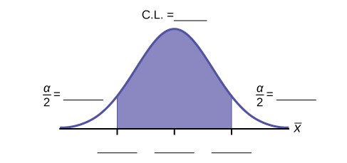
Figure 8.12
- In one complete sentence, explain what the interval means.
- Using the same mean, standard deviation, and level of confidence, suppose that n were 69 instead of 25. Would the error bound become larger or smaller? How do you know?
- Using the same mean, standard deviation, and sample size, how would the error bound change if the confidence level were reduced to 90%? Why?
- Find the value of the sample size needed to if the confidence interval is 90% that the sample proportion and the population proportion are within 4% of each other. The sample proportion is 0.60. Note: Round all fractions up for n.
This OpenStax book is available for free at http://cnx.org/content/col11776/1.33
- Find the value of the sample size needed to if the confidence interval is 95% that the sample proportion and the population proportion are within 2% of each other. The sample proportion is 0.650. Note: Round all fractions up for n.
- Find the value of the sample size needed to if the confidence interval is 96% that the sample proportion and the population proportion are within 5% of each other. The sample proportion is 0.70. Note: Round all fractions up for n.
- Find the value of the sample size needed to if the confidence interval is 90% that the sample proportion and the population proportion are within 1% of each other. The sample proportion is 0.50. Note: Round all fractions up for n.
- Find the value of the sample size needed to if the confidence interval is 94% that the sample proportion and the population proportion are within 2% of each other. The sample proportion is 0.65. Note: Round all fractions up for n.
- Find the value of the sample size needed to if the confidence interval is 95% that the sample proportion and the population proportion are within 4% of each other. The sample proportion is 0.45. Note: Round all fractions up for n.
- Find the value of the sample size needed to if the confidence interval is 90% that the sample proportion and the population proportion are within 2% of each other. The sample proportion is 0.3. Note: Round all fractions up for n.
HOMEWORK
A Confidence Interval for a Population Standard Deviation Unknown, Small Sample Case
- In six packages of “The Flintstones® Real Fruit Snacks” there were five Bam-Bam snack pieces. The total number of snack pieces in the six bags was 68. We wish to calculate a 96% confidence interval for the population proportion of Bam-Bam snack pieces.
- Define the random variables X and P′ in words.
- Which distribution should you use for this problem? Explain your choice
- Calculate p′.
- Construct a 96% confidence interval for the population proportion of Bam-Bam snack pieces per bag.
- State the confidence interval.
- Sketch the graph.
- Calculate the error bound.
- Do you think that six packages of fruit snacks yield enough data to give accurate results? Why or why not?
- A random survey of enrollment at 35 community colleges across the United States yielded the following figures: 6,414; 1,550; 2,109; 9,350; 21,828; 4,300; 5,944; 5,722; 2,825; 2,044; 5,481; 5,200; 5,853; 2,750; 10,012; 6,357; 27,000; 9,414; 7,681; 3,200; 17,500; 9,200; 7,380; 18,314; 6,557; 13,713; 17,768; 7,493; 2,771; 2,861; 1,263; 7,285; 28,165; 5,080; 11,622. Assume the underlying population is normal.
- i.x– =
- sx =
- n =
- n – 1 =
- Define the random variables X and X– in words.
- Which distribution should you use for this problem? Explain your choice.
- Construct a 95% confidence interval for the population mean enrollment at community colleges in the United States.
- State the confidence interval.
- Sketch the graph.
- What will happen to the error bound and confidence interval if 500 community colleges were surveyed? Why?
- Suppose that a committee is studying whether or not there is waste of time in our judicial system. It is interested in the mean amount of time individuals waste at the courthouse waiting to be called for jury duty. The committee randomly surveyed 81 people who recently served as jurors. The sample mean wait time was eight hours with a sample standard deviation of four hours.
- i.x– =
- sx =
- n =
- n – 1 = –
- Define the random variables X and X
in words.
- Which distribution should you use for this problem? Explain your choice.
- Construct a 95% confidence interval for the population mean time wasted.
- State the confidence interval.
- Sketch the graph.
- Explain in a complete sentence what the confidence interval means.
- A pharmaceutical company makes tranquilizers. It is assumed that the distribution for the length of time they last is approximately normal. Researchers in a hospital used the drug on a random sample of nine patients. The effective period of the tranquilizer for each patient (in hours) was as follows: 2.7; 2.8; 3.0; 2.3; 2.3; 2.2; 2.8; 2.1; and 2.4.
- i.x– =
- sx =
- n =
- n – 1 =
- Define the random variable X in words.
- Define the random variable X– in words.
- Which distribution should you use for this problem? Explain your choice.
- Construct a 95% confidence interval for the population mean length of time.
- State the confidence interval.
- Sketch the graph.
- What does it mean to be “95% confident” in this problem?
- Suppose that 14 children, who were learning to ride two-wheel bikes, were surveyed to determine how long they had to use training wheels. It was revealed that they used them an average of six months with a sample standard deviation of three months. Assume that the underlying population distribution is normal.
- i.x– =
- sx =
- n =
- n – 1 =
- Define the random variable X in words.
- Define the random variable X– in words.
- Which distribution should you use for this problem? Explain your choice.
- Construct a 99% confidence interval for the population mean length of time using training wheels.
- State the confidence interval.
- Sketch the graph.
- Why would the error bound change if the confidence level were lowered to 90%?
This OpenStax book is available for free at http://cnx.org/content/col11776/1.33
- The Federal Election Commission (FEC) collects information about campaign contributions and disbursements for candidates and political committees each election cycle. A political action committee (PAC) is a committee formed to raise money for candidates and campaigns. A Leadership PAC is a PAC formed by a federal politician (senator or representative) to raise money to help other candidates’ campaigns.
The FEC has reported financial information for 556 Leadership PACs that operating during the 2011–2012 election cycle. The following table shows the total receipts during this cycle for a random selection of 30 Leadership PACs.
|
$46,500.00 |
$0 |
$40,966.50 |
$105,887.20 |
$5,175.00 |
|
$29,050.00 |
$19,500.00 |
$181,557.20 |
$31,500.00 |
$149,970.80 |
|
$2,555,363.20 |
$12,025.00 |
$409,000.00 |
$60,521.70 |
$18,000.00 |
|
$61,810.20 |
$76,530.80 |
$119,459.20 |
$0 |
$63,520.00 |
|
$6,500.00 |
$502,578.00 |
$705,061.10 |
$708,258.90 |
$135,810.00 |
|
$2,000.00 |
$2,000.00 |
$0 |
$1,287,933.80 |
$219,148.30 |
Table 8.3
x– = $251, 854.23
s = $521, 130.41
Use this sample data to construct a 95% confidence interval for the mean amount of money raised by all Leadership PACs during the 2011–2012 election cycle. Use the Student’s t-distribution.
- Forbes magazine published data on the best small firms in 2012. These were firms that had been publicly traded for at least a year, have a stock price of at least $5 per share, and have reported annual revenue between $5 million and $1 billion. The Table 8.4 shows the ages of the corporate CEOs for a random sample of these firms.
|
58 |
51 |
61 |
56 |
|
|
59 |
74 |
63 |
53 |
50 |
|
59 |
60 |
60 |
57 |
46 |
|
55 |
63 |
57 |
47 |
55 |
|
57 |
43 |
61 |
62 |
49 |
|
67 |
67 |
55 |
55 |
49 |
Table 8.4
Use this sample data to construct a 90% confidence interval for the mean age of CEO’s for these top small firms. Use the Student’s t-distribution.
- Unoccupied seats on flights cause airlines to lose revenue. Suppose a large airline wants to estimate its mean number of unoccupied seats per flight over the past year. To accomplish this, the records of 225 flights are randomly selected and the number of unoccupied seats is noted for each of the sampled flights. The sample mean is 11.6 seats and the sample standard deviation is 4.1 seats.
- i.x– =
- sx =
- n =
- n-1 =
- Define the random variables X and X– in words.
- Which distribution should you use for this problem? Explain your choice.
- Construct a 92% confidence interval for the population mean number of unoccupied seats per flight.
- State the confidence interval.
- Sketch the graph.
- In a recent sample of 84 used car sales costs, the sample mean was $6,425 with a standard deviation of $3,156. Assume the underlying distribution is approximately normal.
- Which distribution should you use for this problem? Explain your choice.
- Define the random variable X– in words.
- Construct a 95% confidence interval for the population mean cost of a used car.
- State the confidence interval.
- Sketch the graph.
- Explain what a “95% confidence interval” means for this study.
- Six different national brands of chocolate chip cookies were randomly selected at the supermarket. The grams of fat per serving are as follows: 8; 8; 10; 7; 9; 9. Assume the underlying distribution is approximately normal.
- Construct a 90% confidence interval for the population mean grams of fat per serving of chocolate chip cookies sold in supermarkets.
- State the confidence interval.
- Sketch the graph.
- If you wanted a smaller error bound while keeping the same level of confidence, what should have been changed in the study before it was done?
- Go to the store and record the grams of fat per serving of six brands of chocolate chip cookies.
- Calculate the mean.
- Is the mean within the interval you calculated in part a? Did you expect it to be? Why or why not?
- A survey of the mean number of cents off that coupons give was conducted by randomly surveying one coupon per page from the coupon sections of a recent San Jose Mercury News. The following data were collected: 20¢; 75¢; 50¢; 65¢; 30¢; 55¢; 40¢; 40¢; 30¢; 55¢; $1.50; 40¢; 65¢; 40¢. Assume the underlying distribution is approximately normal.
- i.x– =
- sx =
- n =
- n-1 =
- Define the random variables X and X– in words.
- Which distribution should you use for this problem? Explain your choice.
- Construct a 95% confidence interval for the population mean worth of coupons.
- State the confidence interval.
- Sketch the graph.
- If many random samples were taken of size 14, what percent of the confidence intervals constructed should contain the population mean worth of coupons? Explain why.
Use the following information to answer the next two exercises: A quality control specialist for a restaurant chain takes a random sample of size 12 to check the amount of soda served in the 16 oz. serving size. The sample mean is 13.30 with a sample standard deviation of 1.55. Assume the underlying population is normally distributed.
- Find the 95% Confidence Interval for the true population mean for the amount of soda served. a. (12.42, 14.18)
b. (12.32, 14.29)
c. (12.50, 14.10)
- Impossible to determine
A Confidence Interval for A Population Proportion
- Insurance companies are interested in knowing the population percent of drivers who always buckle up before riding in a car.
- When designing a study to determine this population proportion, what is the minimum number you would need to survey to be 95% confident that the population proportion is estimated to within 0.03?
- If it were later determined that it was important to be more than 95% confident and a new survey was commissioned, how would that affect the minimum number you would need to survey? Why?
This OpenStax book is available for free at http://cnx.org/content/col11776/1.33
- Suppose that the insurance companies did do a survey. They randomly surveyed 400 drivers and found that 320 claimed they always buckle up. We are interested in the population proportion of drivers who claim they always buckle up.
- i. x =
- n =
- p′ =
- Define the random variables X and P′, in words.
- Which distribution should you use for this problem? Explain your choice.
- Construct a 95% confidence interval for the population proportion who claim they always buckle up.
- State the confidence interval.
- Sketch the graph.
- If this survey were done by telephone, list three difficulties the companies might have in obtaining random results.
- According to a recent survey of 1,200 people, 61% feel that the president is doing an acceptable job. We are interested in the population proportion of people who feel the president is doing an acceptable job.
- Define the random variables X and P′ in words.
- Which distribution should you use for this problem? Explain your choice.
- Construct a 90% confidence interval for the population proportion of people who feel the president is doing an acceptable job.
- State the confidence interval.
- Sketch the graph.
- An article regarding interracial dating and marriage recently appeared in the Washington Post. Of the 1,709 randomly selected adults, 315 identified themselves as Latinos, 323 identified themselves as blacks, 254 identified themselves as Asians, and 779 identified themselves as whites. In this survey, 86% of blacks said that they would welcome a white person into their families. Among Asians, 77% would welcome a white person into their families, 71% would welcome a Latino, and 66% would welcome a black person.
- We are interested in finding the 95% confidence interval for the percent of all black adults who would welcome a white person into their families. Define the random variables X and P′, in words.
- Which distribution should you use for this problem? Explain your choice.
- Construct a 95% confidence interval.
- State the confidence interval.
- Sketch the graph.
- Refer to the information in Exercise 8.117.
- Construct three 95% confidence intervals.
- percent of all Asians who would welcome a white person into their families.
- percent of all Asians who would welcome a Latino into their families.
- percent of all Asians who would welcome a black person into their families.
- Even though the three point estimates are different, do any of the confidence intervals overlap? Which?
- For any intervals that do overlap, in words, what does this imply about the significance of the differences in the true proportions?
- For any intervals that do not overlap, in words, what does this imply about the significance of the differences in the true proportions?
- Stanford University conducted a study of whether running is healthy for men and women over age 50. During the first eight years of the study, 1.5% of the 451 members of the 50-Plus Fitness Association died. We are interested in the proportion of people over 50 who ran and died in the same eight-year period.
- Define the random variables X and P′ in words.
- Which distribution should you use for this problem? Explain your choice.
- Construct a 97% confidence interval for the population proportion of people over 50 who ran and died in the same eight–year period.
- State the confidence interval.
- Sketch the graph.
- Explain what a “97% confidence interval” means for this study.
- A telephone poll of 1,000 adult Americans was reported in an issue of Time Magazine. One of the questions asked was “What is the main problem facing the country?” Twenty percent answered “crime.” We are interested in the population proportion of adult Americans who feel that crime is the main problem.
- Define the random variables X and P′ in words.
- Which distribution should you use for this problem? Explain your choice.
- Construct a 95% confidence interval for the population proportion of adult Americans who feel that crime is the main problem.
- State the confidence interval.
- Sketch the graph.
- Suppose we want to lower the sampling error. What is one way to accomplish that?
- The sampling error given by Yankelovich Partners, Inc. (which conducted the poll) is ±3%. In one to three complete sentences, explain what the ±3% represents.
- Refer to Exercise 8.120. Another question in the poll was “[How much are] you worried about the quality of education in our schools?” Sixty-three percent responded “a lot”. We are interested in the population proportion of adult Americans who are worried a lot about the quality of education in our schools.
- Define the random variables X and P′ in words.
- Which distribution should you use for this problem? Explain your choice.
- Construct a 95% confidence interval for the population proportion of adult Americans who are worried a lot about the quality of education in our schools.
- State the confidence interval.
- Sketch the graph.
- The sampling error given by Yankelovich Partners, Inc. (which conducted the poll) is ±3%. In one to three complete sentences, explain what the ±3% represents.
Use the following information to answer the next three exercises: According to a Field Poll, 79% of California adults (actual results are 400 out of 506 surveyed) feel that “education and our schools” is one of the top issues facing California. We wish to construct a 90% confidence interval for the true proportion of California adults who feel that education and the schools is one of the top issues facing California.
b. 1.27
c. 0.79
d. 400
- A 90% confidence interval for the population proportion is . a. (0.761, 0.820)
b. (0.125, 0.188)
c. (0.755, 0.826)
d. (0.130, 0.183)
Use the following information to answer the next two exercises: Five hundred and eleven (511) homes in a certain southern California community are randomly surveyed to determine if they meet minimal earthquake preparedness recommendations. One hundred seventy-three (173) of the homes surveyed met the minimum recommendations for earthquake preparedness, and 338 did not.
- Find the confidence interval at the 90% Confidence Level for the true population proportion of southern California community homes meeting at least the minimum recommendations for earthquake preparedness.
a. (0.2975, 0.3796)
b. (0.6270, 0.6959)
c. (0.3041, 0.3730)
d. (0.6204, 0.7025)
- The point estimate for the population proportion of homes that do not meet the minimum recommendations for earthquake preparedness is .
a. 0.6614
b. 0.3386
c. 173
d. 338
This OpenStax book is available for free at http://cnx.org/content/col11776/1.33
- On May 23, 2013, Gallup reported that of the 1,005 people surveyed, 76% of U.S. workers believe that they will continue working past retirement age. The confidence level for this study was reported at 95% with a ±3% margin of error.
- Determine the estimated proportion from the sample.
- Determine the sample size.
- Identify CL and α.
- Calculate the error bound based on the information provided.
- Compare the error bound in part d to the margin of error reported by Gallup. Explain any differences between the values.
- Create a confidence interval for the results of this study.
- A reporter is covering the release of this study for a local news station. How should she explain the confidence interval to her audience?
- A national survey of 1,000 adults was conducted on May 13, 2013 by Rasmussen Reports. It concluded with 95% confidence that 49% to 55% of Americans believe that big-time college sports programs corrupt the process of higher education.
- Find the point estimate and the error bound for this confidence interval.
- Can we (with 95% confidence) conclude that more than half of all American adults believe this?
- Use the point estimate from part a and n = 1,000 to calculate a 75% confidence interval for the proportion of American adults that believe that major college sports programs corrupt higher education.
- Can we (with 75% confidence) conclude that at least half of all American adults believe this?
- Public Policy Polling recently conducted a survey asking adults across the U.S. about music preferences. When asked, 80 of the 571 participants admitted that they have illegally downloaded music.
- Create a 99% confidence interval for the true proportion of American adults who have illegally downloaded music.
- This survey was conducted through automated telephone interviews on May 6 and 7, 2013. The error bound of the survey compensates for sampling error, or natural variability among samples. List some factors that could affect the survey’s outcome that are not covered by the margin of error.
- Without performing any calculations, describe how the confidence interval would change if the confidence level changed from 99% to 90%.
- You plan to conduct a survey on your college campus to learn about the political awareness of students. You want to estimate the true proportion of college students on your campus who voted in the 2012 presidential election with 95% confidence and a margin of error no greater than five percent. How many students must you interview?
Calculating the Sample Size n: Continuous and Binary Random Variables
- Among various ethnic groups, the standard deviation of heights is known to be approximately three inches. We wish to construct a 95% confidence interval for the mean height of male Swedes. Forty-eight male Swedes are surveyed. The sample mean is 71 inches. The sample standard deviation is 2.8 inches.
- i.x– =
- σ =
- n = –
- In words, define the random variables X and X .
- Which distribution should you use for this problem? Explain your choice.
- Construct a 95% confidence interval for the population mean height of male Swedes.
- State the confidence interval.
- Sketch the graph.
- What will happen to the level of confidence obtained if 1,000 male Swedes are surveyed instead of 48? Why?
- Announcements for 84 upcoming engineering conferences were randomly picked from a stack of IEEE Spectrum magazines. The mean length of the conferences was 3.94 days, with a standard deviation of 1.28 days. Assume the
underlying population is normal.–
- In words, define the random variables X and X .
- Which distribution should you use for this problem? Explain your choice.
- Construct a 95% confidence interval for the population mean length of engineering conferences.
- State the confidence interval.
- Sketch the graph.
- Suppose that an accounting firm does a study to determine the time needed to complete one person’s tax forms. It randomly surveys 100 people. The sample mean is 23.6 hours. There is a known standard deviation of 7.0 hours. The population distribution is assumed to be normal.
- i.x– =
- σ =
- n =
- In words, define the random variables X and X– .
- Which distribution should you use for this problem? Explain your choice.
- Construct a 90% confidence interval for the population mean time to complete the tax forms.
- State the confidence interval.
- Sketch the graph.
- If the firm wished to increase its level of confidence and keep the error bound the same by taking another survey, what changes should it make?
- If the firm did another survey, kept the error bound the same, and only surveyed 49 people, what would happen to the level of confidence? Why?
- Suppose that the firm decided that it needed to be at least 96% confident of the population mean length of time to within one hour. How would the number of people the firm surveys change? Why?
- A sample of 16 small bags of the same brand of candies was selected. Assume that the population distribution of bag weights is normal. The weight of each bag was then recorded. The mean weight was two ounces with a standard deviation of 0.12 ounces. The population standard deviation is known to be 0.1 ounce.
- i.x– =
- σ =
- sx =
- In words, define the random variable X.
- In words, define the random variable X– .
- Which distribution should you use for this problem? Explain your choice.
- Construct a 90% confidence interval for the population mean weight of the candies.
- State the confidence interval.
- Sketch the graph.
- Construct a 98% confidence interval for the population mean weight of the candies.
- State the confidence interval.
- Sketch the graph.
- Calculate the error bound.
- In complete sentences, explain why the confidence interval in part f is larger than the confidence interval in part e.
- In complete sentences, give an interpretation of what the interval in part f means.
- A camp director is interested in the mean number of letters each child sends during his or her camp session. The population standard deviation is known to be 2.5. A survey of 20 campers is taken. The mean from the sample is 7.9 with a sample standard deviation of 2.8.
- i.x– =
- σ =
- n =
- Define the random variables X and X– in words.
- Which distribution should you use for this problem? Explain your choice.
- Construct a 90% confidence interval for the population mean number of letters campers send home.
- State the confidence interval.
- Sketch the graph.
- What will happen to the error bound and confidence interval if 500 campers are surveyed? Why?
This OpenStax book is available for free at http://cnx.org/content/col11776/1.33
- What is meant by the term “90% confident” when constructing a confidence interval for a mean?
- If we took repeated samples, approximately 90% of the samples would produce the same confidence interval.
- If we took repeated samples, approximately 90% of the confidence intervals calculated from those samples would contain the sample mean.
- If we took repeated samples, approximately 90% of the confidence intervals calculated from those samples would contain the true value of the population mean.
- If we took repeated samples, the sample mean would equal the population mean in approximately 90% of the samples.
- The Federal Election Commission collects information about campaign contributions and disbursements for candidates and political committees each election cycle. During the 2012 campaign season, there were 1,619 candidates for the House of Representatives across the United States who received contributions from individuals. Table 8.5 shows the total receipts from individuals for a random selection of 40 House candidates rounded to the nearest $100. The standard deviation for this data to the nearest hundred is σ = $909,200.
|
$1,243,900 |
$10,900 |
$385,200 |
$581,500 |
|
|
$7,400 |
$2,900 |
$400 |
$3,714,500 |
$632,500 |
|
$391,000 |
$467,400 |
$56,800 |
$5,800 |
$405,200 |
|
$733,200 |
$8,000 |
$468,700 |
$75,200 |
$41,000 |
|
$13,300 |
$9,500 |
$953,800 |
$1,113,500 |
$1,109,300 |
|
$353,900 |
$986,100 |
$88,600 |
$378,200 |
$13,200 |
|
$3,800 |
$745,100 |
$5,800 |
$3,072,100 |
$1,626,700 |
|
$512,900 |
$2,309,200 |
$6,600 |
$202,400 |
$15,800 |
Table 8.5
- Find the point estimate for the population mean.
- Using 95% confidence, calculate the error bound.
- Create a 95% confidence interval for the mean total individual contributions.
- Interpret the confidence interval in the context of the problem.
- The American Community Survey (ACS), part of the United States Census Bureau, conducts a yearly census similar to the one taken every ten years, but with a smaller percentage of participants. The most recent survey estimates with 90% confidence that the mean household income in the U.S. falls between $69,720 and $69,922. Find the point estimate for mean
U.S. household income and the error bound for mean U.S. household income.
- The average height of young adult males has a normal distribution with standard deviation of 2.5 inches. You want to estimate the mean height of students at your college or university to within one inch with 93% confidence. How many male students must you measure?
- If the confidence interval is change to a higher probability, would this cause a lower, or a higher, minimum sample size?
- If the tolerance is reduced by half, how would this affect the minimum sample size?
- If the value of p is reduced, would this necessarily reduce the sample size needed?
- Is it acceptable to use a higher sample size than the one calculated by z2 pq ?
e2
- A company has been running an assembly line with 97.42%% of the products made being acceptable. Then, a critical piece broke down. After the repairs the decision was made to see if the number of defective products made was still close enough to the long standing production quality. Samples of 500 pieces were selected at random, and the defective rate was found to be 0.025%.
- Is this sample size adequate to claim the company is checking within the 90% confidence interval?
- The 95% confidence interval?
REFERENCES
A Confidence Interval for a Population Standard Deviation, Known or Large Sample Size
“American Fact Finder.” U.S. Census Bureau. Available online at http://factfinder2.census.gov/faces/nav/jsf/pages/ searchresults.xhtml?refresh=t (accessed July 2, 2013).
“Disclosure Data Catalog: Candidate Summary Report 2012.” U.S. Federal Election Commission. Available online at http://www.fec.gov/data/index.jsp (accessed July 2, 2013).
“Headcount Enrollment Trends by Student Demographics Ten-Year Fall Trends to Most Recently Completed Fall.” Foothill De Anza Community College District. Available online at http://research.fhda.edu/factbook/FH_Demo_Trends/ FoothillDemographicTrends.htm (accessed September 30,2013).
Kuczmarski, Robert J., Cynthia L. Ogden, Shumei S. Guo, Laurence M. Grummer-Strawn, Katherine M. Flegal, Zuguo Mei, Rong Wei, Lester R. Curtin, Alex F. Roche, Clifford L. Johnson. “2000 CDC Growth Charts for the United States: Methods and Development.” Centers for Disease Control and Prevention. Available online at http://www.cdc.gov/growthcharts/ 2000growthchart-us.pdf (accessed July 2, 2013).
La, Lynn, Kent German. “Cell Phone Radiation Levels.” c|net part of CBX Interactive Inc. Available online at http://reviews.cnet.com/cell-phone-radiation-levels/ (accessed July 2, 2013).
“Mean Income in the Past 12 Months (in 2011 Inflaction-Adjusted Dollars): 2011 American Community Survey 1-Year Estimates.” American Fact Finder, U.S. Census Bureau. Available online at http://factfinder2.census.gov/faces/ tableservices/jsf/pages/productview.xhtml?pid=ACS_11_1YR_S1902&prodType=table (accessed July 2, 2013).
“Metadata Description of Candidate Summary File.” U.S. Federal Election Commission. Available online at http://www.fec.gov/finance/disclosure/metadata/metadataforcandidatesummary.shtml (accessed July 2, 2013).
“National Health and Nutrition Examination Survey.” Centers for Disease Control and Prevention. Available online at http://www.cdc.gov/nchs/nhanes.htm (accessed July 2, 2013).
A Confidence Interval for a Population Standard Deviation Unknown, Small Sample Case
“America’s Best Small Companies.” Forbes, 2013. Available online at http://www.forbes.com/best-small-companies/list/ (accessed July 2, 2013).
Data from Microsoft Bookshelf.
Data from http://www.businessweek.com/. Data from http://www.forbes.com/.
“Disclosure Data Catalog: Leadership PAC and Sponsors Report, 2012.” Federal Election Commission. Available online at http://www.fec.gov/data/index.jsp (accessed July 2,2013).
“Human Toxome Project: Mapping the Pollution in People.” Environmental Working Group. Available online at http://www.ewg.org/sites/humantoxome/participants/participant-group.php?group=in+utero%2Fnewborn (accessed July 2, 2013).
“Metadata Description of Leadership PAC List.” Federal Election Commission. Available online at http://www.fec.gov/ finance/disclosure/metadata/metadataLeadershipPacList.shtml (accessed July 2, 2013).
A Confidence Interval for A Population Proportion
Jensen, Tom. “Democrats, Republicans Divided on Opinion of Music Icons.” Public Policy Polling. Available online at http://www.publicpolicypolling.com/Day2MusicPoll.pdf (accessed July 2, 2013).
Madden, Mary, Amanda Lenhart, Sandra Coresi, Urs Gasser, Maeve Duggan, Aaron Smith, and Meredith Beaton. “Teens, Social Media, and Privacy.” PewInternet, 2013. Available online at http://www.pewinternet.org/Reports/2013/Teens-Social- Media-And-Privacy.aspx (accessed July 2, 2013).
Prince Survey Research Associates International. “2013 Teen and Privacy Management Survey.” Pew Research Center: Internet and American Life Project. Available online at http://www.pewinternet.org/~/media//Files/Questionnaire/2013/ Methods%20and%20Questions_Teens%20and%20Social%20Media.pdf (accessed July 2, 2013).
This OpenStax book is available for free at http://cnx.org/content/col11776/1.33
Saad, Lydia. “Three in Four U.S. Workers Plan to Work Pas Retirement Age: Slightly more say they will do this by choice rather than necessity.” Gallup® Economy, 2013. Available online at http://www.gallup.com/poll/162758/three-four- workers-plan-work-past-retirement-age.aspx (accessed July 2, 2013).
The Field Poll. Available online at http://field.com/fieldpollonline/subscribers/ (accessed July 2, 2013).
Zogby. “New SUNYIT/Zogby Analytics Poll: Few Americans Worry about Emergency Situations Occurring in Their Community; Only one in three have an Emergency Plan; 70% Support Infrastructure ‘Investment’ for National Security.” Zogby Analytics, 2013. Available online at http://www.zogbyanalytics.com/news/299-americans-neither-worried-nor- prepared-in-case-of-a-disaster-sunyit-zogby-analytics-poll (accessed July 2, 2013).
“52% Say Big-Time College Athletics Corrupt Education Process.” Rasmussen Reports, 2013. Available online at http://www.rasmussenreports.com/public_content/lifestyle/sports/may_2013/ 52_say_big_time_college_athletics_corrupt_education_process (accessed July 2, 2013).
SOLUTIONS
2 X is the number of hours a patient waits in the emergency room before being called back to be examined. X– is the mean wait time of 70 patients in the emergency room.
4 CI: (1.3808, 1.6192)
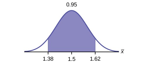
Figure 8.13
EBM = 0.12
- x–
= 151
- sx = 32 c. n = 108
d. n – 1 = 107
8 X– is the mean number of hours spent watching television per month from a sample of 108 Americans.
10 CI: (142.92, 159.08)
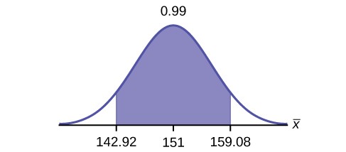
Figure 8.14
EBM = 8.08
a. 3.26
b. 1.02
- 39
14 μ
16 t38
18 0.025
20 (2.93, 3.59)
- We are 95% confident that the true mean number of colors for national flags is between 2.93 colors and 3.59 colors.
- The error bound would become EBM = 0.245. This error bound decreases because as sample sizes increase, variability decreases and we need less interval length to capture the true mean.
26 It would decrease, because the z-score would decrease, which reducing the numerator and lowering the number.
28 X is the number of “successes” where the woman makes the majority of the purchasing decisions for the household. P′ is the percentage of households sampled where the woman makes the majority of the purchasing decisions for the household.
30 CI: (0.5321, 0.6679)
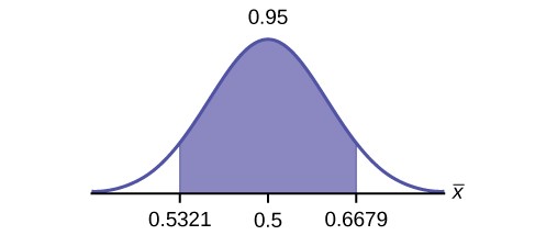
Figure 8.15
EBM: 0.0679
32 X is the number of “successes” where an executive prefers a truck. P′ is the percentage of executives sampled who prefer a truck.
34 CI: (0.19432, 0.33068)
This OpenStax book is available for free at http://cnx.org/content/col11776/1.33
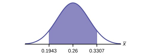
Figure 8.16
36 The sampling error means that the true mean can be 2% above or below the sample mean.
38 P′ is the proportion of voters sampled who said the economy is the most important issue in the upcoming election.
40 CI: (0.62735, 0.67265) EBM: 0.02265
42 The number of girls, ages 8 to 12, in the 5 P.M. Monday night beginning ice-skating class.
- x = 64
- n = 80 c. p′ = 0.8
46 p
48 P′~ N⎛0.8, (0.8)(0.2)⎞ . (0.72171, 0.87829).
⎝
50 0.04
80⎠
52 (0.72; 0.88)
54 With 92% confidence, we estimate the proportion of girls, ages 8 to 12, in a beginning ice-skating class at the Ice Chalet to be between 72% and 88%.
56 The error bound would increase. Assuming all other variables are kept constant, as the confidence level increases, the area under the curve corresponding to the confidence level becomes larger, which creates a wider interval and thus a larger error.
a. 244
- 15
- 50
60 N⎛244, 15 ⎞
⎝50⎠
62 As the sample size increases, there will be less variability in the mean, so the interval size decreases.
64 X is the time in minutes it takes to complete the U.S. Census short form. X– is the mean time it took a sample of 200 people to complete the U.S. Census short form.
66 CI: (7.9441, 8.4559)
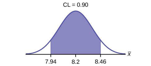
Figure 8.17
68 The level of confidence would decrease because decreasing n makes the confidence interval wider, so at the same error bound, the confidence level decreases.
70–
- x
= 2.2
b. σ = 0.2
c. n = 20
72 X– is the mean weight of a sample of 20 heads of lettuce.
74 EBM = 0.07
CI: (2.1264, 2.2736)
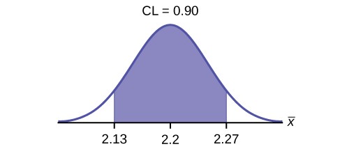
Figure 8.18
76 The interval is greater because the level of confidence increased. If the only change made in the analysis is a change in confidence level, then all we are doing is changing how much area is being calculated for the normal distribution. Therefore, a larger confidence level results in larger areas and larger intervals.
78 The confidence level would increase.
80 30.4
82 σ
84 μ
86 normal
88 0.025
90 (24.52,36.28)
92 We are 95% confident that the true mean age for Winger Foothill College students is between 24.52 and 36.28.
This OpenStax book is available for free at http://cnx.org/content/col11776/1.33
94 The error bound for the mean would decrease because as the CL decreases, you need less area under the normal curve (which translates into a smaller interval) to capture the true population mean.
96 2,185
98 6,765
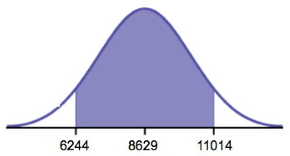 ii.
ii.
Figure 8.19
d. It will become smaller
a.i.x– = 2.51
- sx = 0.318
- n = 9
- n – 1 = 8
- the effective length of time for a tranquilizer
- the mean effective length of time of tranquilizers from a sample of nine patients
- We need to use a Student’s-t distribution, because we do not know the population standard deviation. e.i. CI: (2.27, 2.76)
ii. Check student’s solution.
f. If we were to sample many groups of nine patients, 95% of the samples would contain the true population mean length of time.
107x– = $251, 854.23 s = $521, 130.41 Note that we are not given the population standard deviation, only the standard deviation of the sample. There are 30 measures in the sample, so n = 30, and df = 30 – 1 = 29 CL = 0.96, so α =
1 – CL = 1 – 0.96 = 0.04 α = 0.02t α = t0.02 = 2.150 EBM = t α ⎛ s ⎞ = 2.150⎛521, 130.41⎞
~ $204, 561.66 x– –
222 ⎝ n⎠
⎝30⎠
EBM = $251,854.23 – $204,561.66 = $47,292.57 x– + EBM = $251,854.23+ $204,561.66 = $456,415.89 We estimate with
96% confidence that the mean amount of money raised by all Leadership PACs during the 2011–2012 election cycle lies between $47,292.57 and $456,415.89.
a.i.x– = 11.6
- sx = 4.1
- n = 225
iv. n – 1 = 224
- X is the number of unoccupied seats on a single flight. X– is the mean number of unoccupied seats from a sample of 225 flights.
- We will use a Student’s-t distribution, because we do not know the population standard deviation.
|
d. |
i. ii. |
CI: (11.12 , 12.08) Check student’s solution. |
|
a. |
i. |
CI: (7.64 , 9.36) |
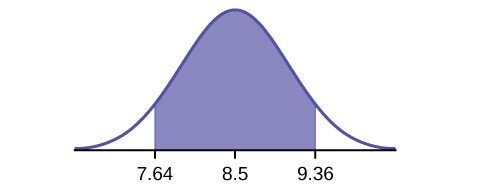 ii.
ii.
Figure 8.20
- The sample should have been increased.
- Answers will vary.
- Answers will vary.
- Answers will vary.
113 b
a. 1,068
b. The sample size would need to be increased since the critical value increases as the confidence level increases.
a. X = the number of people who feel that the president is doing an acceptable job;
P′ = the proportion of people in a sample who feel that the president is doing an acceptable job.
⎛(0.61)(0.39)⎞
b.N⎝0.61,
1200⎠
c.i. CI: (0.59, 0.63)
This OpenStax book is available for free at http://cnx.org/content/col11776/1.33
ii. Check student’s solution
a.i. (0.72, 0.82)
ii. (0.65, 0.76)
iii. (0.60, 0.72)
- Yes, the intervals (0.72, 0.82) and (0.65, 0.76) overlap, and the intervals (0.65, 0.76) and (0.60, 0.72) overlap.
- We can say that there does not appear to be a significant difference between the proportion of Asian adults who say that their families would welcome a white person into their families and the proportion of Asian adults who say that their families would welcome a Latino person into their families.
- We can say that there is a significant difference between the proportion of Asian adults who say that their families would welcome a white person into their families and the proportion of Asian adults who say that their families would welcome a black person into their families.
- X = the number of adult Americans who feel that crime is the main problem; P′ = the proportion of adult Americans who feel that crime is the main problem
- N⎝0.2, (0.2)(0.8)⎠ .
Sin⎛ce we are estim⎞ating a proportion, given P′ = 0.2 and n = 1000, the distribution we should use is
1000
c.i. CI: (0.18, 0.22)
ii. Check student’s solution.
- One way to lower the sampling error is to increase the sample size.
- The stated “± 3%” represents the maximum error bound. This means that those doing the study are reporting a maximum error of 3%. Thus, they estimate the percentage of adult Americans who feel that crime is the main problem to be between 18% and 22%.
122 c
125 a
a. p′ = (0.55 + 0.49)
2
= 0.52; EBP = 0.55 – 0.52 = 0.03
- No, the confidence interval includes values less than or equal to 0.50. It is possible that less than half of the population believe this.
- CL = 0.75, so α = 1 – 0.75 = 0.25 and α = 0.125 z α = 1.150 . (The area to the right of this z is 0.125, so the area to
22
0.52(0.48)1, 000
the left is 1 – 0.125 = 0.875.)
EBP = (1.150)≈ 0.018
(p′ – EBP, p′ + EBP) = (0.52 – 0.018, 0.52 + 0.018) = (0.502, 0.538)
- Yes – this interval does not fall less than 0.50 so we can conclude that at least half of all American adults believe that major sports programs corrupt education – but we do so with only 75% confidence.
- i. 71
- 2.8
- 48
- X is the height of a male Swede, and x is the mean height from a sample of 48 male Swedes.
- Normal. We know the standard deviation for the population, and the sample size is greater than 30. d.i. CI: (70.151, 71.85)
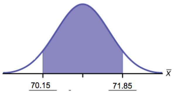 ii.
ii.
Figure 8.21
e. The confidence interval will decrease in size, because the sample size increased. Recall, when all factors remain unchanged, an increase in sample size decreases variability. Thus, we do not need as large an interval to capture the true population mean.
a.i.x– = 23.6
- σ = 7
- n = 100
- X is the time needed to complete an individual tax form. X– is the mean time to complete tax forms from a sample of 100 customers.
- N⎛23.6, 7 ⎞ because we know sigma.
⎝100⎠
d.i. (22.228, 24.972)
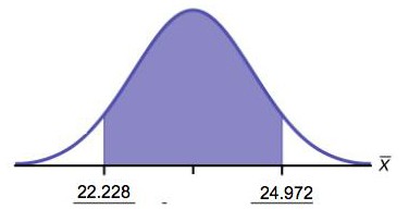 ii.
ii.
Figure 8.22
- It will need to change the sample size. The firm needs to determine what the confidence level should be, then apply the error bound formula to determine the necessary sample size.
This OpenStax book is available for free at http://cnx.org/content/col11776/1.33
- The confidence level would increase as a result of a larger interval. Smaller sample sizes result in more variability. To capture the true population mean, we need to have a larger interval.
- According to the error bound formula, the firm needs to survey 206 people. Since we increase the confidence level, we need to increase either our error bound or the sample size.
a.i. 7.9
- 2.5
- 20
b. X is the number of letters a single camper will send home. X– is the mean number of letters sent home from a sample of 20 campers.
c. N 7.9⎛ 2.5 ⎞
⎝ 20⎠
d.i. CI: (6.98, 8.82)
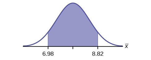 ii.
ii.
Figure 8.23
e. The error bound and confidence interval will decrease.
136 –
a.x
= $568,873
b. CL = 0.95 α = 1 – 0.95 = 0.05 z α
2
= 1.96
n
EBM = z0.025 σ
= 1.96 909200
40
= $281,764
c.x– − EBM = 568,873 − 281,764 = 287,109
x– + EBM = 568,873 + 281,764 = 850,637
d. We estimate with 95% confidence that the mean amount of contributions received from all individuals by House candidates is between $287,109 and $850,637.
- Higher
- It would increase to four times the prior value.
- No, It could have no affect if it were to change to 1 – p, for example. If it gets closer to 0.5 the minimum sample size would increase.
- Yes
- No
- No
This OpenStax book is available for free at http://cnx.org/content/col11776/1.33