12 12 | F DISTRIBUTION AND ONE-WAY ANOVA

Figure 12.1 One-way ANOVA is used to measure information from several groups.

Introduction

Many statistical applications in psychology, social science, business administration, and the natural sciences involve several groups. For example, an environmentalist is interested in knowing if the average amount of pollution varies in several bodies of water. A sociologist is interested in knowing if the amount of income a person earns varies according to his or her upbringing. A consumer looking for a new car might compare the average gas mileage of several models.

For hypothesis tests comparing averages among more than two groups, statisticians have developed a method called “Analysis of Variance” (abbreviated ANOVA). In this chapter, you will study the simplest form of ANOVA called single factor or one-way ANOVA. You will also study the F distribution, used for one-way ANOVA, and the test for differences between two variances. This is just a very brief overview of one-way ANOVA. One-Way ANOVA, as it is presented here, relies heavily on a calculator or computer.

| Test of Two Variances

This chapter introduces a new probability density function, the F distribution. This distribution is used for many applications

including ANOVA and for testing equality across multiple means. We begin with the F distribution and the test of hypothesis of differences in variances. It is often desirable to compare two variances rather than two averages. For instance, college administrators would like two college professors grading exams to have the same variation in their grading. In order for a lid to fit a container, the variation in the lid and the container should be approximately the same. A supermarket might be interested in the variability of check-out times for two checkers. In finance, the variance is a measure of risk and thus an interesting question would be to test the hypothesis that two different investment portfolios have the same variance, the volatility.

In order to perform a F test of two variances, it is important that the following are true:

• The populations from which the two samples are drawn are approximately normally distributed.
• The two populations are independent of each other.

Unlike most other hypothesis tests in this book, the F test for equality of two variances is very sensitive to deviations from normality. If the two distributions are not normal, or close, the test can give a biased result for the test statistic.

Suppose we sample randomly from two independent normal populations. Let σ 2 and σ 2 be the unknown population

12

variances and s2 and s2 be the sample variances. Let the sample sizes be n1 and n2. Since we are interested in comparing

12

the two sample variances, we use the F ratio:

⎡s12 ⎤

⎢⎥

2
F = ⎣σ1 ⎦

⎡s22 ⎤

⎢⎥

2
⎣σ2 ⎦

F has the distribution F ~ F(n1 – 1, n2 – 1)

where n1 – 1 are the degrees of freedom for the numerator and n2 – 1 are the degrees of freedom for the denominator.

⎡s12 ⎤

⎢

2
If the null hypothesis is σ 2 = σ 2 , then the F Ratio, test statistic, becomes Fc = ⎣σ1

⎥

⎦ = s12

12⎡s22 ⎤

s22

The various forms of the hypotheses tested are:

⎢⎥

2
⎣σ2 ⎦

Table 12.1

A more general form of the null and alternative hypothesis for a two tailed test would be :

H : σ12 = δ

0 σ220

a2
H : σ12 ≠ δ

σ20

Where if δ0 = 1 it is a simple test of the hypothesis that the two variances are equal. This form of the hypothesis does have the benefit of allowing for tests that are more than for simple differences and can accommodate tests for specific differences as we did for differences in means and differences in proportions. This form of the hypothesis also shows the relationship between the F distribution and the χ2 : the F is a ratio of two chi squared distributions a distribution we saw in the last chapter. This is helpful in determining the degrees of freedom of the resultant F distribution.

This OpenStax book is available for free at http://cnx.org/content/col11776/1.33

If the two populations have equal variances, then s2 and s2 are close in value and the test statistic, F

= s12

is close to

12c

s22

one. But if the two population variances are very different, s2 and s2 tend to be very different, too. Choosing s2 as the

121

larger sample variance causes the ratio s12

to be greater than one. If s2 and s2 are far apart, then F

= s12

is a large

number.

s22

12c

s22

Therefore, if F is close to one, the evidence favors the null hypothesis (the two population variances are equal). But if F is much larger than one, then the evidence is against the null hypothesis. In essence, we are asking if the calculated F statistic, test statistic, is significantly different from one.

To determine the critical points we have to find Fα,df1,df2. See Appendix A for the F table. This F table has values for various levels of significance from 0.1 to 0.001 designated as “p” in the first column. To find the critical value choose the desired significance level and follow down and across to find the critical value at the intersection of the two different degrees of freedom. The F distribution has two different degrees of freedom, one associated with the numerator, df1, and one associated with the denominator, df2 and to complicate matters the F distribution is not symmetrical and changes the degree of skewness as the degrees of freedom change. The degrees of freedom in the numerator is n1-1, where n1 is the sample size for group 1, and the degrees of freedom in the denominator is n2-1, where n2 is the sample size for group 2. Fα,df1,df2 will give the critical value on the upper end of the F distribution.

To find the critical value for the lower end of the distribution, reverse the degrees of freedom and divide the F-value from the table into one.

Upper tail critical value : Fα,df1,df2 Lower tail critical value : 1/Fα,df2,df1

When the calculated value of F is between the critical values, not in the tail, we cannot reject the null hypothesis that the two variances came from a population with the same variance. If the calculated F-value is in either tail we cannot accept the null hypothesis just as we have been doing for all of the previous tests of hypothesis.

An alternative way of finding the critical values of the F distribution makes the use of the F-table easier. We note in the F-table that all the values of F are greater than one therefore the critical F value for the left hand tail will always be less than one because to find the critical value on the left tail we divide an F value into the number one as shown above. We also note that if the sample variance in the numerator of the test statistic is larger than the sample variance in the denominator, the resulting F value will be greater than one. The shorthand method for this test is thus to be sure that the larger of the two sample variances is placed in the numerator to calculate the test statistic. This will mean that only the right hand tail critical value will have to be found in the F-table.

Example 12.1Two college instructors are interested in whether or not there is any variation in the way they grade math exams. They each grade the same set of 10 exams. The first instructor’s grades have a variance of 52.3. The second instructor’s grades have a variance of 89.9. Test the claim that the first instructor’s variance is smaller. (In most colleges, it is desirable for the variances of exam grades to be nearly the same among instructors.) The level of significance is 10%.Solution 12.1Let 1 and 2 be the subscripts that indicate the first and second instructor, respectively.n1 = n2 = 10.H0: σ 2 ≥ σ 2 and Ha: σ 2 < σ 21212Calculate the test statistic: By the null hypothesis (σ 2 ≥ σ 2 ) , the F statistic is:12F = s22 = 89.9 = 1.719cs1252.3

Critical value for the test: F9,9 = 5.35 where n1 – 1 = 9 and n2 – 1 = 9.

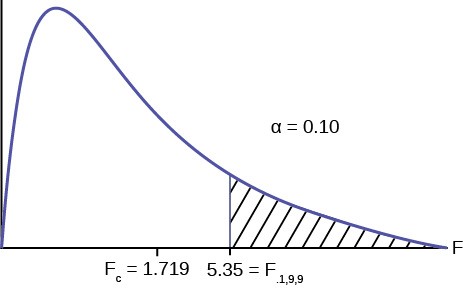
Figure 12.2

Make a decision: Since the calculated F value is not in the tail we cannot reject H0.

12.1 The New York Choral Society divides male singers up into four categories from highest voices to lowest: Tenor1, Tenor2, Bass1, Bass2. In the table are heights of the men in the Tenor1 and Bass2 groups. One suspects that taller men will have lower voices, and that the variance of height may go up with the lower voices as well. Do we have good evidence that the variance of the heights of singers in each of these two groups (Tenor1 and Bass2) are different?Table 12.2
Conclusion: With a 10% level of significance, from the data, there is insufficient evidence to conclude that the variance in grades for the first instructor is smaller.

This OpenStax book is available for free at http://cnx.org/content/col11776/1.33

| One-Way ANOVA

The purpose of a one-way ANOVA test is to determine the existence of a statistically significant difference among several group means. The test actually uses variances to help determine if the means are equal or not. In order to perform a one- way ANOVA test, there are five basic assumptions to be fulfilled:

• Each population from which a sample is taken is assumed to be normal.
• All samples are randomly selected and independent.
• The populations are assumed to have equal standard deviations (or variances).
• The factor is a categorical variable.
• The response is a numerical variable.

The Null and Alternative Hypotheses

The null hypothesis is simply that all the group population means are the same. The alternative hypothesis is that at least one pair of means is different. For example, if there are k groups:

H0 : µ 1 = µ 2 = µ 3 = . . .µk

Ha : At least two of the group means µ 1, µ 2, µ 3, . . . ,µk are not equal. That is, µi ≠µ j for some i≠j .

The graphs, a set of box plots representing the distribution of values with the group means indicated by a horizontal line through the box, help in the understanding of the hypothesis test. In the first graph (red box plots), H0: μ1 = μ2 = μ3 and the three populations have the same distribution if the null hypothesis is true. The variance of the combined data is approximately the same as the variance of each of the populations.

If the null hypothesis is false, then the variance of the combined data is larger which is caused by the different means as shown in the second graph (green box plots).

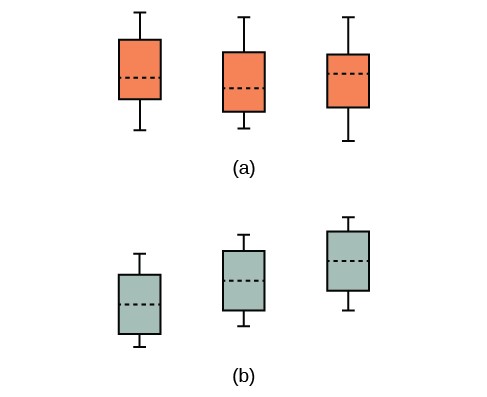
Figure 12.3 (a) H0 is true. All means are the same; the differences are due to random variation. (b) H0 is not true. All means are not the same; the differences are too large to be due to random variation.

| The F Distribution and the F-Ratio

The distribution used for the hypothesis test is a new one. It is called the F distribution, invented by George Snedecor but named in honor of Sir Ronald Fisher, an English statistician. The F statistic is a ratio (a fraction). There are two sets of degrees of freedom; one for the numerator and one for the denominator.

For example, if F follows an F distribution and the number of degrees of freedom for the numerator is four, and the number of degrees of freedom for the denominator is ten, then F ~ F4,10.

To calculate the F ratio, two estimates of the variance are made.

• Variance between samples: An estimate of σ2 that is the variance of the sample means multiplied by n (when the sample sizes are the same.). If the samples are different sizes, the variance between samples is weighted to account for the different sample sizes. The variance is also called variation due to treatment or explained variation.
• Variance within samples: An estimate of σ2 that is the average of the sample variances (also known as a pooled variance). When the sample sizes are different, the variance within samples is weighted. The variance is also called the variation due to error or unexplained variation.
• SSbetween = the sum of squares that represents the variation among the different samples
• SSwithin = the sum of squares that represents the variation within samples that is due to chance.

To find a “sum of squares” means to add together squared quantities that, in some cases, may be weighted. We used sum of squares to calculate the sample variance and the sample standard deviation in Section 2..

MS means ” mean square.” MSbetween is the variance between groups, and MSwithin is the variance within groups.

Calculation of Sum of Squares and Mean Square

• k = the number of different groups
• nj = the size of the jth group
• sj = the sum of the values in the jth group
• n = total number of all the values combined (total sample size: ∑nj)
• x = one value: ∑x = ∑sj
• Sum of squares of all values from every group combined: ∑x2

⎛∑ x2⎞

• Between group variability: SStotal = ∑x2 – ⎝ n ⎠

∑ x
⎛⎞2

• Total sum of squares: ∑x2 –

⎝⎠

n

• Explained variation: sum of squares representing variation among the different samples:

⎣
−
⎦
⎡(s j)2⎤(∑ s j)2

SSbetween = ∑ ⎢ n j ⎥n

• Unexplainedvariation:sumofsquaresrepresentingvariationwithinsamplesduetochance:

SSwithin = SStotal – SSbetween

• df‘s for different groups (df‘s for the numerator): df = k – 1
• Equation for errors within samples (df‘s for the denominator): dfwithin = n – k
• Mean square (variance estimate) explained by the different groups: MSbetween = SSbetween

d fbetween

• Mean square (variance estimate) that is due to chance (unexplained): MSwithin = SSwithin

d fwithin

MSbetween and MSwithin can be written as follows:

• MSbetween = SSbetween = SSbetween

d fbetweenk − 1

• MSwithin = SSwithin = SSwithin

d fwithinn − k

The one-way ANOVA test depends on the fact that MSbetween can be influenced by population differences among means of the several groups. Since MSwithin compares values of each group to its own group mean, the fact that group means might be different does not affect MSwithin.

This OpenStax book is available for free at http://cnx.org/content/col11776/1.33

NOTEThe null hypothesis says that all the group population means are equal. The hypothesis of equal means implies that the populations have the same normal distribution, because it is assumed that the populations are normal and that they have equal variances.
The null hypothesis says that all groups are samples from populations having the same normal distribution. The alternate hypothesis says that at least two of the sample groups come from populations with different normal distributions. If the null hypothesis is true, MSbetween and MSwithin should both estimate the same value.

F-Ratio or F Statistic

F =
MSbetween MSwithin

If MSbetween and MSwithin estimate the same value (following the belief that H0 is true), then the F-ratio should be approximately equal to one. Mostly, just sampling errors would contribute to variations away from one. As it turns out, MSbetween consists of the population variance plus a variance produced from the differences between the samples. MSwithin is an estimate of the population variance. Since variances are always positive, if the null hypothesis is false, MSbetween will generally be larger than MSwithin.Then the F-ratio will be larger than one. However, if the population effect is small, it is not unlikely that MSwithin will be larger in a given sample.

The foregoing calculations were done with groups of different sizes. If the groups are the same size, the calculations simplify somewhat and the F-ratio can be written as:

atio Formula when the groups are the same size

F = n ⋅ s –x 2

s2 pooled

where …

• n = the sample size
• dfnumerator = k – 1
• dfdenominator = n – k
• s2 pooled = the mean of the sample variances (pooled variance)
• s –x 2 = the variance of the sample means

Data are typically put into a table for easy viewing. One-Way ANOVA results are often displayed in this manner by computer software.

Table 12.3

Example 12.2Three different diet plans are to be tested for mean weight loss. The entries in the table are the weight losses for the different plans. The one-way ANOVA results are shown in Table 12.4.

Table 12.4

s1 = 16.5, s2 =15, s3 = 15.5

Following are the calculations needed to fill in the one-way ANOVA table. The table is used to conduct a hypothesis test.

⎡(s )2⎤

⎛∑ s ⎞2

⎣
−
n j
n
⎦
SS(between) = ∑ ⎢ j ⎥⎝j⎠

s
2

=1 +

22

s
s
2 + 3 −

(s1

+ s2

+ s3)2

43310

where n1 = 4, n2 = 3, n3 = 3 and n = n1 + n2 + n3 = 10

= (16.5)2 + (15)2 + (15.5)2 − (16.5 + 15 + 15.5)2

43310

SS(between) = 2.2458

⎛∑ x⎞2

S(total) = ∑ x2 − ⎝ n ⎠

= ⎛52 + 4.52 + 42 + 32 + 3.52 + 72 + 4.52 + 82 + 42 + 3.52⎞

⎝⎠

−
(5 + 4.5 + 4 + 3 + 3.5 + 7 + 4.5 + 8 + 4 + 3.5)2

10

10
= 244 − 472 = 244 − 220.9

SS(total) = 23.1

SS(within) = SS(total) − SS(between)

=23.1 − 2.2458

SS(within) = 20.8542

This OpenStax book is available for free at http://cnx.org/content/col11776/1.33

Table 12.5

12.2 As part of an experiment to see how different types of soil cover would affect slicing tomato production, Marist College students grew tomato plants under different soil cover conditions. Groups of three plants each had one of the following treatmentsbare soila commercial ground coverblack plasticstrawcompostAll plants grew under the same conditions and were the same variety. Students recorded the weight (in grams) of tomatoes produced by each of the n = 15 plants:Table 12.6Create the one-way ANOVA table.
The one-way ANOVA hypothesis test is always right-tailed because larger F-values are way out in the right tail of the

F-distribution curve and tend to make us reject H0.

Example 12.3Let’s return to the slicing tomato exercise in Try It. The means of the tomato yields under the five mulching conditions are represented by μ1, μ2, μ3, μ4, μ5. We will conduct a hypothesis test to determine if all means are the same or at least one is different. Using a significance level of 5%, test the null hypothesis that there is no difference in mean yields among the five groups against the alternative hypothesis that at least one mean is different from the rest.

Solution 12.3

The null and alternative hypotheses are:

H0: μ1 = μ2 = μ3 = μ4 = μ5

Ha: μi ≠ μj some i ≠ j

The one-way ANOVA results are shown in Table 12.6

Table 12.7

Distribution for the test: F4,10

df(num) = 5 – 1 = 4

df(denom) = 15 – 5 = 10

Test statistic: F = 4.4810

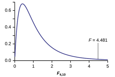
Figure 12.4

Probability Statement: p-value = P(F > 4.481) = 0.0248. Compare α and the p-value: α = 0.05, p-value = 0.0248 Make a decision: Since α > p-value, we cannot accept H0.

Conclusion: At the 5% significance level, we have reasonably strong evidence that differences in mean yields for

slicing tomato plants grown under different mulching conditions are unlikely to be due to chance alone. We may conclude that at least some of mulches led to different mean yields.

This OpenStax book is available for free at http://cnx.org/content/col11776/1.33

12.3 MRSA, or Staphylococcus aureus, can cause a serious bacterial infections in hospital patients. Table 12.8 shows various colony counts from different patients who may or may not have MRSA. The data from the table is plotted in Figure 12.5.Table 12.8Plot of the data for the different concentrations:Figure 12.5Test whether the mean number of colonies are the same or are different. Construct the ANOVA table, find the p-value, and state your conclusion. Use a 5% significance level.
Example 12.4Four sororities took a random sample of sisters regarding their grade means for the past term. The results are shown in Table 12.9.Table 12.9 MEAN GRADES FOR FOUR SORORITIES

Table 12.9 MEAN GRADES FOR FOUR SORORITIES

Using a significance level of 1%, is there a difference in mean grades among the sororities?

Solution 12.4

NOTEThis is an example of a balanced design, because each factor (i.e., sorority) has the same number of observations.
Let μ1, μ2, μ3, μ4 be the population means of the sororities. Remember that the null hypothesis claims that the sorority groups are from the same normal distribution. The alternate hypothesis says that at least two of the sorority groups come from populations with different normal distributions. Notice that the four sample sizes are each five.

H0: µ 1 = µ 2 = µ 3 = µ 4

Ha: Not all of the means µ 1, µ 2, µ 3, µ 4 are equal.

Distribution for the test: F3,16

where k = 4 groups and n = 20 samples in total

df(num)= k – 1 = 4 – 1 = 3

df(denom) = n – k = 20 – 4 = 16 Calculate the test statistic: F = 2.23 Graph:

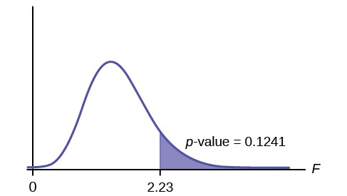
Figure 12.6

Probability statement: p-value = P(F > 2.23) = 0.1241

Compare α and the p-value: α = 0.01

This OpenStax book is available for free at http://cnx.org/content/col11776/1.33

Example 12.5A fourth grade class is studying the environment. One of the assignments is to grow bean plants in different soils. Tommy chose to grow his bean plants in soil found outside his classroom mixed with dryer lint. Tara chose to grow her bean plants in potting soil bought at the local nursery. Nick chose to grow his bean plants in soil from his mother’s garden. No chemicals were used on the plants, only water. They were grown inside the classroom next to a large window. Each child grew five plants. At the end of the growing period, each plant was measured, producing the data (in inches) in Table 12.11.Table 12.11Does it appear that the three media in which the bean plants were grown produce the same mean height? Test at a 3% level of significance.

p-value = 0.1241

α < p-value

Make a decision: Since α < p-value, you cannot reject H0.

12.4 Four sports teams took a random sample of players regarding their GPAs for the last year. The results are shown in Table 12.10.Table 12.10 GPAs FOR FOUR SPORTS TEAMSUse a significance level of 5%, and determine if there is a difference in GPA among the teams.
Conclusion: There is not sufficient evidence to conclude that there is a difference among the mean grades for the sororities.

Solution 12.5

This time, we will perform the calculations that lead to the F’ statistic. Notice that each group has the same

number of plants, so we will use the formula F‘ = n ⋅ s –x 2 .

s2 pooled

First, calculate the sample mean and sample variance of each group.

Table 12.12

Next, calculate the variance of the three group means (Calculate the variance of 24.2, 25.4, and 24.4). Variance of the group means = 0.413 = s –x 2

Then MSbetween = ns –x 2 = (5)(0.413) where n = 5 is the sample size (number of plants each child grew).

Calculate the mean of the three sample variances (Calculate the mean of 11.7, 18.3, and 16.3). Mean of the sample variances = 15.433 = s2 pooled

Then MSwithin = s2pooled = 15.433.

The F statistic (or F ratio) is F = MSbetween = ns –x 2

= (5)(0.413) = 0.134

MSwithin

s2 pooled

15.433

The dfs for the numerator = the number of groups – 1 = 3 – 1 = 2.

The dfs for the denominator = the total number of samples – the number of groups = 15 – 3 = 12 The distribution for the test is F2,12 and the F statistic is F = 0.134

The p-value is P(F > 0.134) = 0.8759.

Decision: Since α = 0.03 and the p-value = 0.8759, then you cannot reject H0. (Why?)

Conclusion: With a 3% level of significance, from the sample data, the evidence is not sufficient to conclude that the mean heights of the bean plants are different.

Notation

The notation for the F distribution is F ~ Fdf(num),df(denom)

where df(num) = dfbetween and df(denom) = dfwithin

(denom) –
The mean for the F distribution is µ = d f d f (num) 2

| Facts About the F Distribution

Here are some facts about the F distribution.

• The curve is not symmetrical but skewed to the right.
• There is a different curve for each set of degrees of freedom.
• The F statistic is greater than or equal to zero.
• As the degrees of freedom for the numerator and for the denominator get larger, the curve approximates the normal as

This OpenStax book is available for free at http://cnx.org/content/col11776/1.33

can be seen in the two figures below. Figure (b) with more degrees of freedom is more closely approaching the normal distribution, but remember that the F cannot ever be less than zero so the distribution does not have a tail that goes to infinity on the left as the normal distribution does.

• Other uses for the F distribution include comparing two variances and two-way Analysis of Variance. Two-Way Analysis is beyond the scope of this chapter.

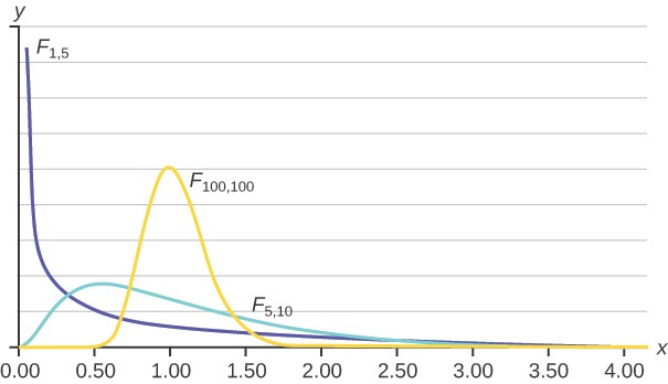
Figure 12.7

KEY TERMS

Analysis of Variance also referred to as ANOVA, is a method of testing whether or not the means of three or more populations are equal. The method is applicable if:

• all populations of interest are normally distributed.
• the populations have equal standard deviations.
• samples (not necessarily of the same size) are randomly and independently selected from each population.
• there is one independent variable and one dependent variable. The test statistic for analysis of variance is the F-ratio.

One-Way ANOVA a method of testing whether or not the means of three or more populations are equal; the method is applicable if:

• all populations of interest are normally distributed.
• the populations have equal standard deviations.
• samples (not necessarily of the same size) are randomly and independently selected from each population. The test statistic for analysis of variance is the F-ratio.

Variance mean of the squared deviations–from the mean; the square of the stand–ard deviation. For a set of data, a

deviation can be represented as x – x where x is a value of the data and x is the sample mean. The sample

variance is equal to the sum of the squares of the deviations divided by the difference of the sample size and one.

CHAPTER REVIEW

Test of Two Variances

The F test for the equality of two variances rests heavily on the assumption of normal distributions. The test is unreliable if this assumption is not met. If both distributions are normal, then the ratio of the two sample variances is distributed as an F statistic, with numerator and denominator degrees of freedom that are one less than the samples sizes of the corresponding two groups. A test of two variances hypothesis test determines if two variances are the same. The distribution for the hypothesis test is the F distribution with two different degrees of freedom.

Assumptions:

• The populations from which the two samples are drawn are normally distributed.
• The two populations are independent of each other.

One-Way ANOVA

Analysis of variance extends the comparison of two groups to several, each a level of a categorical variable (factor). Samples from each group are independent, and must be randomly selected from normal populations with equal variances. We test the null hypothesis of equal means of the response in every group versus the alternative hypothesis of one or more group means being different from the others. A one-way ANOVA hypothesis test determines if several population means are equal. The distribution for the test is the F distribution with two different degrees of freedom.

Assumptions:

• Each population from which a sample is taken is assumed to be normal.
• All samples are randomly selected and independent.
• The populations are assumed to have equal standard deviations (or variances).

The F Distribution and the F-Ratio

Analysis of variance compares the means of a response variable for several groups. ANOVA compares the variation within each group to the variation of the mean of each group. The ratio of these two is the F statistic from an F distribution with (number of groups – 1) as the numerator degrees of freedom and (number of observations – number of groups) as the

This OpenStax book is available for free at http://cnx.org/content/col11776/1.33

denominator degrees of freedom. These statistics are summarized in the ANOVA table.

Facts About the F Distribution

The graph of the F distribution is always positive and skewed right, though the shape can be mounded or exponential depending on the combination of numerator and denominator degrees of freedom. The F statistic is the ratio of a measure of the variation in the group means to a similar measure of the variation within the groups. If the null hypothesis is correct, then the numerator should be small compared to the denominator. A small F statistic will result, and the area under the F curve to the right will be large, representing a large p-value. When the null hypothesis of equal group means is incorrect, then the numerator should be large compared to the denominator, giving a large F statistic and a small area (small p-value) to the right of the statistic under the F curve.

When the data have unequal group sizes (unbalanced data), then techniques from Section 12.3 need to be used for hand calculations. In the case of balanced data (the groups are the same size) however, simplified calculations based on group means and variances may be used. In practice, of course, software is usually employed in the analysis. As in any analysis, graphs of various sorts should be used in conjunction with numerical techniques. Always look at your data!

FORMULA REVIEW

12.1 Test of Two Variances

σ 2

SSwithin = SStotal − SSbetween

dfbetween = df(num) = k – 1

= δ0σ
2
H0 : 1

1 ≠ δ0σ
2
2

dfwithin

= df(denom) = n – k

SSbetween

Ha : σ

MSbetween =

d fbetween

2
2

if δ0=1 then

MSwithin =

SSwithin d fwithin

H0 : σ 2 = σ 2

MSbetween

12F =

1
Ha : σ 2 ≠ σ2

Test statistic is :

S
2
c1
F = S2 2

12.3 The F Distribution and the F-Ratio

⎛⎞2

MSwithin

• k = the number of groups
• nj = the size of the jth group
• sj = the sum of the values in the jth group
• n = the total number of all values (observations) combined
• x = one value (one observation) from the data

⎡(s j)2⎤

⎝∑ s j⎠

• 
  s –x 2 = the variance of the sample means

⎣
−
⎦
SSbetween = ∑ ⎢ n j ⎥n

• s2

pooled

= the mean of the sample variances (pooled

⎛∑ x⎞2

variance)

SStotal = ∑ x2 − ⎝ n ⎠

PRACTICE

Test of Two Variances

Use the following information to answer the next two exercises. There are two assumptions that must be true in order to perform an F test of two variances.

• Name one assumption that must be true.
• What is the other assumption that must be true?

Use the following information to answer the next five exercises. Two coworkers commute from the same building. They are interested in whether or not there is any variation in the time it takes them to drive to work. They each record their times for 20 commutes. The first worker’s times have a variance of 12.1. The second worker’s times have a variance of 16.9. The first worker thinks that he is more consistent with his commute times. Test the claim at the 10% level. Assume that commute times are normally distributed.

• State the null and alternative hypotheses.
• What is s1 in this problem?
• What is s2 in this problem?
• What is n?
• What is the F statistic?
• What is the critical value?
• Is the claim accurate?

Use the following information to answer the next four exercises. Two students are interested in whether or not there is variation in their test scores for math class. There are 15 total math tests they have taken so far. The first student’s grades have a standard deviation of 38.1. The second student’s grades have a standard deviation of 22.5. The second student thinks his scores are more consistent.

• State the null and alternative hypotheses.
• What is the F Statistic?
• What is the critical value?
• At the 5% significance level, do we reject the null hypothesis?

Use the following information to answer the next three exercises. Two cyclists are comparing the variances of their overall paces going uphill. Each cyclist records his or her speeds going up 35 hills. The first cyclist has a variance of 23.8 and the second cyclist has a variance of 32.1. The cyclists want to see if their variances are the same or different. Assume that commute times are normally distributed.

• State the null and alternative hypotheses.
• What is the F Statistic?
• At the 5% significance level, what can we say about the cyclists’ variances?

One-Way ANOVA

Use the following information to answer the next five exercises. There are five basic assumptions that must be fulfilled in order to perform a one-way ANOVA test. What are they?

• Write one assumption.
• Write another assumption.
• Write a third assumption.
• Write a fourth assumption.

The F Distribution and the F-Ratio

Use the following information to answer the next eight exercises. Groups of men from three different areas of the country are to be tested for mean weight. The entries in Table 12.13 are the weights for the different groups.

Table 12.13

This OpenStax book is available for free at http://cnx.org/content/col11776/1.33

Table 12.13

• What is the Sum of Squares Factor?
• What is the Sum of Squares Error?
• What is the df for the numerator?
• What is the df for the denominator?
• What is the Mean Square Factor?
• What is the Mean Square Error?
• What is the F statistic?

Use the following information to answer the next eight exercises. Girls from four different soccer teams are to be tested for mean goals scored per game. The entries in Table 12.14 are the goals per game for the different teams.

Table 12.14

• What is SSbetween?
• What is the df for the numerator?
• What is MSbetween?
• What is SSwithin?
• What is the df for the denominator?
• What is MSwithin?
• What is the F statistic?
• Judging by the F statistic, do you think it is likely or unlikely that you will reject the null hypothesis?

Facts About the F Distribution

• An F statistic can have what values?
• What happens to the curves as the degrees of freedom for the numerator and the denominator get larger?

Use the following information to answer the next seven exercise. Four basketball teams took a random sample of players regarding how high each player can jump (in inches). The results are shown in Table 12.15.

Table 12.15

• What is the df(num)?
• What is the df(denom)?
• What are the Sum of Squares and Mean Squares Factors?
• What are the Sum of Squares and Mean Squares Errors?
• What is the F statistic?
• What is the p-value?
• At the 5% significance level, is there a difference in the mean jump heights among the teams?

Use the following information to answer the next seven exercises. A video game developer is testing a new game on three different groups. Each group represents a different target market for the game. The developer collects scores from a random sample from each group. The results are shown in Table 12.16

Table 12.16

• What is the df(num)?
• What is the df(denom)?
• What are the SSbetween and MSbetween?
• What are the SSwithin and MSwithin?
• What is the F Statistic?
• What is the p-value?
• At the 10% significance level, are the scores among the different groups different?

Use the following information to answer the next three exercises. Suppose a group is interested in determining whether teenagers obtain their drivers licenses at approximately the same average age across the country. Suppose that the following data are randomly collected from five teenagers in each region of the country. The numbers represent the age at which teenagers obtained their drivers licenses.

Table 12.17

This OpenStax book is available for free at http://cnx.org/content/col11776/1.33

Table 12.17

Enter the data into your calculator or computer.

• p-value =

State the decisions and conclusions (in complete sentences) for the following preconceived levels of α.

53. α = 0.05

• Decision:
• Conclusion:

54. α = 0.01

• Decision:
• Conclusion:

HOMEWORK

Test of Two Variances

• Three students, Linda, Tuan, and Javier, are given five laboratory rats each for a nutritional experiment. Each rat’s weight is recorded in grams. Linda feeds her rats Formula A, Tuan feeds his rats Formula B, and Javier feeds his rats Formula C. At the end of a specified time period, each rat is weighed again and the net gain in grams is recorded.

Table 12.18

Determine whether or not the variance in weight gain is statistically the same among Javier’s and Linda’s rats. Test at a significance level of 10%.

• A grassroots group opposed to a proposed increase in the gas tax claimed that the increase would hurt working-class people the most, since they commute the farthest to work. Suppose that the group randomly surveyed 24 individuals and asked them their daily one-way commuting mileage. The results are as follows.

Table 12.19

Determine whether or not the variance in mileage driven is statistically the same among the working class and professional (middle income) groups. Use a 5% significance level.

Use the following information to answer the next two exercises. The following table lists the number of pages in four different types of magazines.

Table 12.20

• Which two magazine types do you think have the same variance in length?
• Which two magazine types do you think have different variances in length?

This OpenStax book is available for free at http://cnx.org/content/col11776/1.33

• Is the variance for the amount of money, in dollars, that shoppers spend on Saturdays at the mall the same as the variance for the amount of money that shoppers spend on Sundays at the mall? Suppose that the Table 12.21 shows the results of a study.

Table 12.21

• Are the variances for incomes on the East Coast and the West Coast the same? Suppose that Table 12.22 shows the results of a study. Income is shown in thousands of dollars. Assume that both distributions are normal. Use a level of significance of 0.05.

Table 12.22

• Thirty men in college were taught a method of finger tapping. They were randomly assigned to three groups of ten, with each receiving one of three doses of caffeine: 0 mg, 100 mg, 200 mg. This is approximately the amount in no, one, or two cups of coffee. Two hours after ingesting the caffeine, the men had the rate of finger tapping per minute recorded. The experiment was double blind, so neither the recorders nor the students knew which group they were in. Does caffeine affect the rate of tapping, and if so how?

Here are the data:

Table 12.23

• King Manuel I, Komnenus ruled the Byzantine Empire from Constantinople (Istanbul) during the years 1145 to 1180

A.D. The empire was very powerful during his reign, but declined significantly afterwards. Coins minted during his era were found in Cyprus, an island in the eastern Mediterranean Sea. Nine coins were from his first coinage, seven from the second, four from the third, and seven from a fourth. These spanned most of his reign. We have data on the silver content of the coins:

Table 12.24

Did the silver content of the coins change over the course of Manuel’s reign? Here are the means and variances of each coinage. The data are unbalanced.

Table 12.25

This OpenStax book is available for free at http://cnx.org/content/col11776/1.33

• The American League and the National League of Major League Baseball are each divided into three divisions: East, Central, and West. Many years, fans talk about some divisions being stronger (having better teams) than other divisions. This may have consequences for the postseason. For instance, in 2012 Tampa Bay won 90 games and did not play in the postseason, while Detroit won only 88 and did play in the postseason. This may have been an oddity, but is there good evidence that in the 2012 season, the American League divisions were significantly different in overall records? Use the following data to test whether the mean number of wins per team in the three American League divisions were the same or not. Note that the data are not balanced, as two divisions had five teams, while one had only four.

Table 12.26

Table 12.27

Table 12.28

One-Way ANOVA

• Three different traffic routes are tested for mean driving time. The entries in the Table 12.29 are the driving times in minutes on the three different routes.

Table 12.29

State SSbetween, SSwithin, and the F statistic.

• Suppose a group is interested in determining whether teenagers obtain their drivers licenses at approximately the same average age across the country. Suppose that the following data are randomly collected from five teenagers in each region of the country. The numbers represent the age at which teenagers obtained their drivers licenses.

Table 12.30

State the hypotheses.

H0:

Ha:

The F Distribution and the F-Ratio

Use the following information to answer the next three exercises. Suppose a group is interested in determining whether teenagers obtain their drivers licenses at approximately the same average age across the country. Suppose that the following data are randomly collected from five teenagers in each region of the country. The numbers represent the age at which teenagers obtained their drivers licenses.

Table 12.31

This OpenStax book is available for free at http://cnx.org/content/col11776/1.33

Table 12.31

H0: µ1 = µ2 = µ3 = µ4 = µ5

Hα: At least any two of the group means µ1, µ2, …, µ5 are not equal.

• degrees of freedom – numerator: df(num) =
• degrees of freedom – denominator: df(denom) =
• F statistic =

Facts About the F Distribution

• Three students, Linda, Tuan, and Javier, are given five laboratory rats each for a nutritional experiment. Each rat’s weight is recorded in grams. Linda feeds her rats Formula A, Tuan feeds his rats Formula B, and Javier feeds his rats Formula C. At the end of a specified time period, each rat is weighed again, and the net gain in grams is recorded. Using a significance level of 10%, test the hypothesis that the three formulas produce the same mean weight gain.

Table 12.32 Weights of Student Lab Rats

• A grassroots group opposed to a proposed increase in the gas tax claimed that the increase would hurt working-class people the most, since they commute the farthest to work. Suppose that the group randomly surveyed 24 individuals and asked them their daily one-way commuting mileage. The results are in Table 12.33. Using a 5% significance level, test the hypothesis that the three mean commuting mileages are the same.

Table 12.33

Use the following information to answer the next two exercises. Table 12.34 lists the number of pages in four different

types of magazines.

Table 12.34

• Using a significance level of 5%, test the hypothesis that the four magazine types have the same mean length.
• Eliminate one magazine type that you now feel has a mean length different from the others. Redo the hypothesis test, testing that the remaining three means are statistically the same. Use a new solution sheet. Based on this test, are the mean lengths for the remaining three magazines statistically the same?
• A researcher wants to know if the mean times (in minutes) that people watch their favorite news station are the same. Suppose that Table 12.35 shows the results of a study.

Table 12.35

Assume that all distributions are normal, the four population standard deviations are approximately the same, and the data were collected independently and randomly. Use a level of significance of 0.05.

This OpenStax book is available for free at http://cnx.org/content/col11776/1.33

• Are the means for the final exams the same for all statistics class delivery types? Table 12.36 shows the scores on final exams from several randomly selected classes that used the different delivery types.

Table 12.36

Assume that all distributions are normal, the four population standard deviations are approximately the same, and the data were collected independently and randomly. Use a level of significance of 0.05.

• Are the mean number of times a month a person eats out the same for whites, blacks, Hispanics and Asians? Suppose that Table 12.37 shows the results of a study.

Table 12.37

Assume that all distributions are normal, the four population standard deviations are approximately the same, and the data were collected independently and randomly. Use a level of significance of 0.05.

• Are the mean numbers of daily visitors to a ski resort the same for the three types of snow conditions? Suppose that

Table 12.38 shows the results of a study.

Table 12.38

Assume that all distributions are normal, the four population standard deviations are approximately the same, and the data were collected independently and randomly. Use a level of significance of 0.05.

• Sanjay made identical paper airplanes out of three different weights of paper, light, medium and heavy. He made four airplanes from each of the weights, and launched them himself across the room. Here are the distances (in meters) that his planes flew.

Table 12.39

Figure 12.8

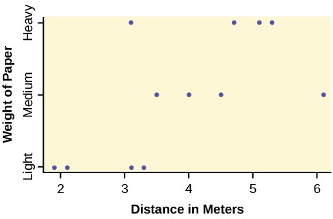
• Take a look at the data in the graph. Look at the spread of data for each group (light, medium, heavy). Does it seem reasonable to assume a normal distribution with the same variance for each group? Yes or No.
• Why is this a balanced design?
• Calculate the sample mean and sample standard deviation for each group.
• Does the weight of the paper have an effect on how far the plane will travel? Use a 1% level of significance. Complete the test using the method shown in the bean plant example in Figure 12.8.
• variance of the group means
• MSbetween=
• mean of the three sample variances
• MSwithin =
• F statistic =
• df(num) = , df(denom) =
• number of groups
• number of observations

◦ p-value = (P(F > ) = )

• Graph the p-value.
• decision:
• conclusion:

This OpenStax book is available for free at http://cnx.org/content/col11776/1.33

• DDT is a pesticide that has been banned from use in the United States and most other areas of the world. It is quite effective, but persisted in the environment and over time became seen as harmful to higher-level organisms. Famously, egg shells of eagles and other raptors were believed to be thinner and prone to breakage in the nest because of ingestion of DDT in the food chain of the birds.

An experiment was conducted on the number of eggs (fecundity) laid by female fruit flies. There are three groups of flies. One group was bred to be resistant to DDT (the RS group). Another was bred to be especially susceptible to DDT (SS). Finally there was a control line of non-selected or typical fruitflies (NS). Here are the data:

Table 12.40

The values are the average number of eggs laid daily for each of 75 flies (25 in each group) over the first 14 days of their lives. Using a 1% level of significance, are the mean rates of egg selection for the three strains of fruitfly different? If so, in what way? Specifically, the researchers were interested in whether or not the selectively bred strains were different from the nonselected line, and whether the two selected lines were different from each other.

Here is a chart of the three groups:

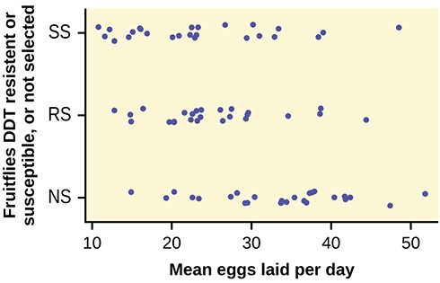
Figure 12.9

• The data shown is the recorded body temperatures of 130 subjects as estimated from available histograms.

Traditionally we are taught that the normal human body temperature is 98.6 F. This is not quite correct for everyone. Are the mean temperatures among the four groups different?

Calculate 95% confidence intervals for the mean body temperature in each group and comment about the confidence intervals.

Table 12.41

REFERENCES

12.1 Test of Two Variances

“MLB Vs. Division Standings – 2012.” Available online at http://espn.go.com/mlb/standings/_/year/2012/type/vs-division/ order/true.

The F Distribution and the F-Ratio

Tomato Data, Marist College School of Science (unpublished student research)

Facts About the F Distribution

Data from a fourth grade classroom in 1994 in a private K – 12 school in San Jose, CA.

Hand, D.J., F. Daly, A.D. Lunn, K.J. McConway, and E. Ostrowski. A Handbook of Small Datasets: Data for Fruitfly Fecundity. London: Chapman & Hall, 1994.

This OpenStax book is available for free at http://cnx.org/content/col11776/1.33

Hand, D.J., F. Daly, A.D. Lunn, K.J. McConway, and E. Ostrowski. A Handbook of Small Datasets. London: Chapman & Hall, 1994, pg. 50.

Hand, D.J., F. Daly, A.D. Lunn, K.J. McConway, and E. Ostrowski. A Handbook of Small Datasets. London: Chapman & Hall, 1994, pg. 118.

“MLB Standings – 2012.” Available online at http://espn.go.com/mlb/standings/_/year/2012.

Mackowiak, P. A., Wasserman, S. S., and Levine, M. M. (1992), “A Critical Appraisal of 98.6 Degrees F, the Upper Limit of the Normal Body Temperature, and Other Legacies of Carl Reinhold August Wunderlich,” Journal of the American Medical Association, 268, 1578-1580.

SOLUTIONS

1 The populations from which the two samples are drawn are normally distributed.

3 H0 : σ1 = σ2 Ha : σ1 < σ2 or H0: σ 2 = σ 2 Ha: σ 2 < σ 2

1212

5 4.11

7 0.7159

9 No, at the 10% level of significance, we cannot reject the null hypothesis and state that the data do not show that the variation in drive times for the first worker is less than the variation in drive times for the second worker.

11 2.8674

13 Cannot accept the null hypothesis. There is enough evidence to say that the variance of the grades for the first student is higher than the variance in the grades for the second student.

15 0.7414

17 Each population from which a sample is taken is assumed to be normal.

19 The populations are assumed to have equal standard deviations (or variances).

21 4,939.2

23 2

25 2,469.6

27 3.7416

29 3

31 13.2

33 0.825

35 Because a one-way ANOVA test is always right-tailed, a high F statistic corresponds to a low p-value, so it is likely that we cannot accept the null hypothesis.

37 The curves approximate the normal distribution.

39 ten

41 SS = 237.33; MS = 23.73

43 0.1614

45 two

47 SS = 5,700.4; MS = 2,850.2

49 3.6101

51 Yes, there is enough evidence to show that the scores among the groups are statistically significant at the 10% level.

55

a.H0 : σ 2 = σ 2

12

b.Ha : σ 2 ≠ σ 2

11

• df(num) = 4; df(denom) = 4
• F4, 4

e. 3.00

• Check student’t solution.
• Decision: Cannot reject the null hypothesis; Conclusion: There is insufficient evidence to conclude that the variances are different.

58 The answers may vary. Sample answer: Home decorating magazines and news magazines have different variances.

60

a. H0: = σ 2 = σ 2

12

b. Ha: σ 2 ≠ σ 2

11

c. df(n) = 7, df(d) = 6

d. F7,6

e. 0.8117

f. 0.7825

• Check student’s solution.
• i. Alpha: 0.05
• Decision: Cannot reject the null hypothesis.
• Reason for decision: calculated test statistics is not in the tail of the distribution
• Conclusion: There is not sufficient evidence to conclude that the variances are different.

• Here is a strip chart of the silver content of the coins:

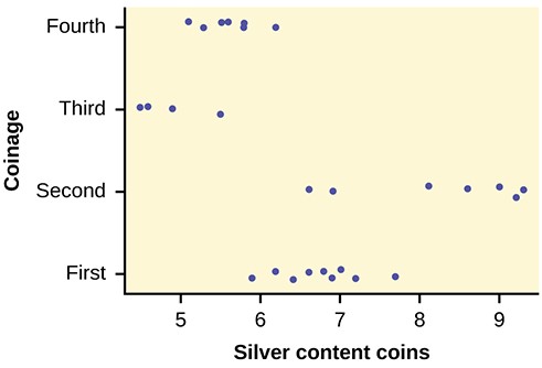
Figure 12.10

While there are differences in spread, it is not unreasonable to use ANOVA techniques. Here is the completed ANOVA table:

This OpenStax book is available for free at http://cnx.org/content/col11776/1.33

Table 12.42

P(F > 26.272) = 0; Cannot accept the null hypothesis for any alpha. There is sufficient evidence to conclude that the mean silver content among the four coinages are different. From the strip chart, it appears that the first and second coinages had higher silver contents than the third and fourth.

• Here is a stripchart of the number of wins for the 14 teams in the AL for the 2012 season.

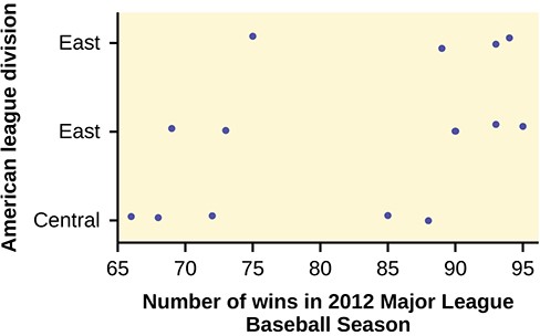
Figure 12.11

While the spread seems similar, there may be some question about the normality of the data, given the wide gaps in the middle near the 0.500 mark of 82 games (teams play 162 games each season in MLB). However, one-way ANOVA is robust. Here is the ANOVA table for the data:

Table 12.43

P(F > 1.5521) = 0.2548

Since the p-value is so large, there is not good evidence against the null hypothesis of equal means. We cannot reject the null hypothesis. Thus, for 2012, there is not any have any good evidence of a significant difference in mean number of wins between the divisions of the American League.

• SSbetween = 26

SSwithin = 441

F = 0.2653

67 df(denom) = 15

69

a. H0: µL = µT = µJ

• Ha: at least any two of the means are different
• df(num) = 2; df(denom) = 12
• F distribution e. 0.67

f. 0.5305

• Check student’s solution.
• Decision:Cannot reject null hypothesis; Conclusion: There is insufficient evidence to conclude that the means are different.

72

• Ha: µc = µn = µh
• At least any two of the magazines have different mean lengths.
• df(num) = 2, df(denom) = 12
• F distribtuion e. F = 15.28
• p-value = 0.001
• Check student’s solution.
• i. Alpha: 0.05
• Decision: Cannot accept the null hypothesis.
• Reason for decision: p-value < alpha
• Conclusion: There is sufficient evidence to conclude that the mean lengths of the magazines are different.

74

a. H0: μo = μh = μf

b. At least two of the means are different. c. df(n) = 2, df(d) = 13

d. F2,13

e. 0.64

f. 0.5437

• Check student’s solution.
• i. Alpha: 0.05
• Decision: Cannot reject the null hypothesis.
• Reason for decision: p-value > alpha
• Conclusion: The mean scores of different class delivery are not different.

76

a. H0: μp = μm = μh

b. At least any two of the means are different. c. df(n) = 2, df(d) = 12

d. F2,12

e. 3.13

f. 0.0807

This OpenStax book is available for free at http://cnx.org/content/col11776/1.33

• Check student’s solution.
• i. Alpha: 0.05
• Decision: Cannot reject the null hypothesis.
• Reason for decision: p-value > alpha
• Conclusion: There is not sufficient evidence to conclude that the mean numbers of daily visitors are different.

78 The data appear normally distributed from the chart and of similar spread. There do not appear to be any serious outliers, so we may proceed with our ANOVA calculations, to see if we have good evidence of a difference between the three groups. H0 : µ1 = µ2 = µ3 ; Ha : µi ≠ ; some i ≠ j Define μ1, μ2, μ3, as the population mean number of eggs laid

by the three groups of fruit flies. F statistic = 8.6657; p-value = 0.0004

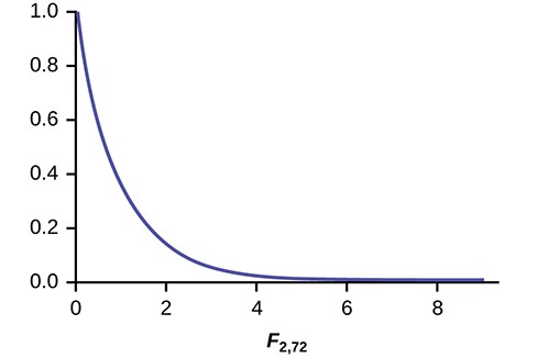
Figure 12.12

Decision: Since the p-value is less than the level of significance of 0.01, we reject the null hypothesis. Conclusion: We have good evidence that the average number of eggs laid during the first 14 days of life for these three strains of fruitflies are different. Interestingly, if you perform a two sample t-test to compare the RS and NS groups they are significantly different (p = 0.0013). Similarly, SS and NS are significantly different (p = 0.0006). However, the two selected groups, RS and SS are not significantly different (p = 0.5176). Thus we appear to have good evidence that selection either for resistance or for susceptibility involves a reduced rate of egg production (for these specific strains) as compared to flies that were not selected for resistance or susceptibility to DDT. Here, genetic selection has apparently involved a loss of fecundity.

This OpenStax book is available for free at http://cnx.org/content/col11776/1.33