9 9 | HYPOTHESIS TESTING WITH ONE SAMPLE

Figure 9.1 You can use a hypothesis test to decide if a dog breeder’s claim that every Dalmatian has 35 spots is statistically sound. (Credit: Robert Neff)

Introduction

Now we are down to the bread and butter work of the statistician: developing and testing hypotheses. It is important to put this material in a broader context so that the method by which a hypothesis is formed is understood completely. Using textbook examples often clouds the real source of statistical hypotheses.

Statistical testing is part of a much larger process known as the scientific method. This method was developed more than two centuries ago as the accepted way that new knowledge could be created. Until then, and unfortunately even today, among some, “knowledge” could be created simply by some authority saying something was so, ipso dicta. Superstition and conspiracy theories were (are?) accepted uncritically.

The scientific method, briefly, states that only by following a careful and specific process can some assertion be included in the accepted body of knowledge. This process begins with a set of assumptions upon which a theory, sometimes called a model, is built. This theory, if it has any validity, will lead to predictions; what we call hypotheses.

As an example, in Microeconomics the theory of consumer choice begins with certain assumption concerning human

behavior. From these assumptions a theory of how consumers make choices using indifference curves and the budget line. This theory gave rise to a very important prediction, namely, that there was an inverse relationship between price and quantity demanded. This relationship was known as the demand curve. The negative slope of the demand curve is really just a prediction, or a hypothesis, that can be tested with statistical tools.

Unless hundreds and hundreds of statistical tests of this hypothesis had not confirmed this relationship, the so-called Law of Demand would have been discarded years ago. This is the role of statistics, to test the hypotheses of various theories to determine if they should be admitted into the accepted body of knowledge; how we understand our world. Once admitted, however, they may be later discarded if new theories come along that make better predictions.

Not long ago two scientists claimed that they could get more energy out of a process than was put in. This caused a tremendous stir for obvious reasons. They were on the cover of Time and were offered extravagant sums to bring their research work to private industry and any number of universities. It was not long until their work was subjected to the rigorous tests of the scientific method and found to be a failure. No other lab could replicate their findings. Consequently they have sunk into obscurity and their theory discarded. It may surface again when someone can pass the tests of the hypotheses required by the scientific method, but until then it is just a curiosity. Many pure frauds have been attempted over time, but most have been found out by applying the process of the scientific method.

This discussion is meant to show just where in this process statistics falls. Statistics and statisticians are not necessarily in the business of developing theories, but in the business of testing others’ theories. Hypotheses come from these theories based upon an explicit set of assumptions and sound logic. The hypothesis comes first, before any data are gathered. Data do not create hypotheses; they are used to test them. If we bear this in mind as we study this section the process of forming and testing hypotheses will make more sense.

One job of a statistician is to make statistical inferences about populations based on samples taken from the population. Confidence intervals are one way to estimate a population parameter. Another way to make a statistical inference is to make a decision about the value of a specific parameter. For instance, a car dealer advertises that its new small truck gets 35 miles per gallon, on average. A tutoring service claims that its method of tutoring helps 90% of its students get an A or a B. A company says that women managers in their company earn an average of $60,000 per year.

A statistician will make a decision about these claims. This process is called ” hypothesis testing.” A hypothesis test involves collecting data from a sample and evaluating the data. Then, the statistician makes a decision as to whether or not there is sufficient evidence, based upon analyses of the data, to reject the null hypothesis.

In this chapter, you will conduct hypothesis tests on single means and single proportions. You will also learn about the errors associated with these tests.

| Null and Alternative Hypotheses

The actual test begins by considering two hypotheses. They are called the null hypothesis and the alternative hypothesis. These hypotheses contain opposing viewpoints.

H0: The null hypothesis: It is a statement of no difference between a sample mean or proportion and a population mean or proportion. In other words, the difference equals 0. This can often be considered the status quo and as a result if you cannot accept the null it requires some action.

Ha: The alternative hypothesis: It is a claim about the population that is contradictory to H0 and what we conclude when we cannot accept H0. The alternative hypothesis is the contender and must win with significant evidence to overthrow the status quo. This concept is sometimes referred to the tyranny of the status quo because as we will see later, to overthrow the null hypothesis takes usually 90 or greater confidence that this is the proper decision.

Since the null and alternative hypotheses are contradictory, you must examine evidence to decide if you have enough evidence to reject the null hypothesis or not. The evidence is in the form of sample data.

After you have determined which hypothesis the sample supports, you make a decision. There are two options for a decision. They are “cannot accept H0” if the sample information favors the alternative hypothesis or “do not reject H0” or “decline to reject H0” if the sample information is insufficient to reject the null hypothesis. These conclusions are all based upon a level of probability, a significance level, that is set my the analyst.

Table 9.1 presents the various hypotheses in the relevant pairs. For example, if the null hypothesis is equal to some value, the alternative has to be not equal to that value.

This OpenStax book is available for free at http://cnx.org/content/col11776/1.33

Table 9.1

NOTEAs a mathematical convention H0 always has a symbol with an equal in it. Ha never has a symbol with an equal in it. The choice of symbol depends on the wording of the hypothesis test.
Example 9.1H0: No more than 30% of the registered voters in Santa Clara County voted in the primary election. p ≤ 30Ha: More than 30% of the registered voters in Santa Clara County voted in the primary election. p > 30
Example 9.2We want to test whether the mean GPA of students in American colleges is different from 2.0 (out of 4.0). The null and alternative hypotheses are:H0: μ = 2.0Ha: μ ≠ 2.0
Example 9.3We want to test if college students take less than five years to graduate from college, on the average. The null and alternative hypotheses are:H0: μ ≥ 5Ha: μ < 5

| Outcomes and the Type I and Type II Errors

When you perform a hypothesis test, there are four possible outcomes depending on the actual truth (or falseness) of the null hypothesis H0 and the decision to reject or not. The outcomes are summarized in the following table:

Table 9.2

The four possible outcomes in the table are:

• The decision is cannot reject H0 when H0 is true (correct decision).

• The decision is cannot accept H0 when H0 is true (incorrect decision known as a Type I error). This case is described as “rejecting a good null”. As we will see later, it is this type of error that we will guard against by setting the probability of making such an error. The goal is to NOT take an action that is an error.
• The decision is cannot reject H0 when, in fact, H0 is false (incorrect decision known as a Type II error). This is called “accepting a false null”. In this situation you have allowed the status quo to remain in force when it should be overturned. As we will see, the null hypothesis has the advantage in competition with the alternative.
• The decision is cannot accept H0 when H0 is false (correct decision).

Each of the errors occurs with a particular probability. The Greek letters α and β represent the probabilities.

α = probability of a Type I error = P(Type I error) = probability of rejecting the null hypothesis when the null hypothesis is true: rejecting a good null.

β = probability of a Type II error = P(Type II error) = probability of not rejecting the null hypothesis when the null hypothesis is false. (1 − β) is called the Power of the Test.

α and β should be as small as possible because they are probabilities of errors.

Statistics allows us to set the probability that we are making a Type I error. The probability of making a Type I error is α. Recall that the confidence intervals in the last unit were set by choosing a value called Zα (or tα) and the alpha value determined the confidence level of the estimate because it was the probability of the interval failing to capture the true mean (or proportion parameter p). This alpha and that one are the same.

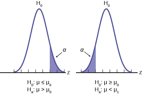
The easiest way to see the relationship between the alpha error and the level of confidence is with the following figure.

Figure 9.2

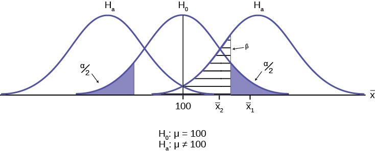
In the center of Figure 9.2 is a normally distributed sampling distribution marked H0. This is a sampling distribution of

X– and by the Central Limit Theorem it is normally distributed. The distribution in the center is marked H0 and represents

the distribution for the null hypotheses H0: µ = 100. This is the value that is being tested. The formal statements of the null and alternative hypotheses are listed below the figure.

The distributions on either side of the H0 distribution represent distributions that would be true if H0 is false, under the alternative hypothesis listed as Ha. We do not know which is true, and will never know. There are, in fact, an infinite number of distributions from which the data could have been drawn if Ha is true, but only two of them are on Figure 9.2 representing all of the others.

To test a hypothesis we take a sample from the population and determine if it could have come from the hypothesized distribution with an acceptable level of significance. This level of significance is the alpha error and is marked on Figure

• as the shaded areas in each tail of the H0 distribution. (Each area is actually α/2 because the distribution is symmetrical and the alternative hypothesis allows for the possibility for the value to be either greater than or less than the hypothesized value–called a two-tailed test).

If the sample mean marked as X– 1 is in the tail of the distribution of H0, we conclude that the probability that it could have

come from the H0 distribution is less than alpha. We consequently state, “the null hypothesis cannot be accepted with (α) level of significance”. The truth may be that this X– 1 did come from the H0 distribution, but from out in the tail. If this is

so then we have falsely rejected a true null hypothesis and have made a Type I error. What statistics has done is provide an

This OpenStax book is available for free at http://cnx.org/content/col11776/1.33

estimate about what we know, and what we control, and that is the probability of us being wrong, α.

We can also see in Figure 9.2 that the sample mean could be really from an Ha distribution, but within the boundary set by the alpha level. Such a case is marked as X– 2 . There is a probability that X– 2 actually came from Ha but shows up in the

range of H0 between the two tails. This probability is the beta error, the probability of accepting a false null.

Our problem is that we can only set the alpha error because there are an infinite number of alternative distributions from which the mean could have come that are not equal to H0. As a result, the statistician places the burden of proof on the alternative hypothesis. That is, we will not reject a null hypothesis unless there is a greater than 90, or 95, or even 99 percent probability that the null is false: the burden of proof lies with the alternative hypothesis. This is why we called this the tyranny of the status quo earlier.

By way of example, the American judicial system begins with the concept that a defendant is “presumed innocent”. This is the status quo and is the null hypothesis. The judge will tell the jury that they can not find the defendant guilty unless the evidence indicates guilt beyond a “reasonable doubt” which is usually defined in criminal cases as 95% certainty of guilt. If the jury cannot accept the null, innocent, then action will be taken, jail time. The burden of proof always lies with the alternative hypothesis. (In civil cases, the jury needs only to be more than 50% certain of wrongdoing to find culpability, called “a preponderance of the evidence”).

The example above was for a test of a mean, but the same logic applies to tests of hypotheses for all statistical parameters one may wish to test.

The following are examples of Type I and Type II errors.

Example 9.4Suppose the null hypothesis, H0, is: Frank’s rock climbing equipment is safe.Type I error: Frank thinks that his rock climbing equipment may not be safe when, in fact, it really is safe.Type II error: Frank thinks that his rock climbing equipment may be safe when, in fact, it is not safe.α = probability that Frank thinks his rock climbing equipment may not be safe when, in fact, it really is safe. β = probability that Frank thinks his rock climbing equipment may be safe when, in fact, it is not safe.Notice that, in this case, the error with the greater consequence is the Type II error. (If Frank thinks his rock climbing equipment is safe, he will go ahead and use it.)This is a situation described as “accepting a false null”.
Example 9.5Suppose the null hypothesis, H0, is: The victim of an automobile accident is alive when he arrives at the emergency room of a hospital. This is the status quo and requires no action if it is true. If the null hypothesis cannot be accepted then action is required and the hospital will begin appropriate procedures.Type I error: The emergency crew thinks that the victim is dead when, in fact, the victim is alive. Type II error: The emergency crew does not know if the victim is alive when, in fact, the victim is dead.α = probability that the emergency crew thinks the victim is dead when, in fact, he is really alive = P(Type I error). β = probability that the emergency crew does not know if the victim is alive when, in fact, the victim is dead = P(Type II error).The error with the greater consequence is the Type I error. (If the emergency crew thinks the victim is dead, they will not treat him.)
9.5 Suppose the null hypothesis, H0, is: a patient is not sick. Which type of error has the greater consequence, Type I

or Type II?

Example 9.6It’s a Boy Genetic Labs claim to be able to increase the likelihood that a pregnancy will result in a boy being born. Statisticians want to test the claim. Suppose that the null hypothesis, H0, is: It’s a Boy Genetic Labs has no effect on gender outcome. The status quo is that the claim is false. The burden of proof always falls to the person making the claim, in this case the Genetics Lab.Type I error: This results when a true null hypothesis is rejected. In the context of this scenario, we would state that we believe that It’s a Boy Genetic Labs influences the gender outcome, when in fact it has no effect. The probability of this error occurring is denoted by the Greek letter alpha, α.Type II error: This results when we fail to reject a false null hypothesis. In context, we would state that It’s a Boy Genetic Labs does not influence the gender outcome of a pregnancy when, in fact, it does. The probability of this error occurring is denoted by the Greek letter beta, β.The error of greater consequence would be the Type I error since couples would use the It’s a Boy Genetic Labs product in hopes of increasing the chances of having a boy.
9.6 “Red tide” is a bloom of poison-producing algae–a few different species of a class of plankton called dinoflagellates. When the weather and water conditions cause these blooms, shellfish such as clams living in the area develop dangerous levels of a paralysis-inducing toxin. In Massachusetts, the Division of Marine Fisheries (DMF) monitors levels of the toxin in shellfish by regular sampling of shellfish along the coastline. If the mean level of toxin in clams exceeds 800 μg (micrograms) of toxin per kg of clam meat in any area, clam harvesting is banned there until the bloom is over and levels of toxin in clams subside. Describe both a Type I and a Type II error in this context, and state which error has the greater consequence.
Example 9.7A certain experimental drug claims a cure rate of at least 75% for males with prostate cancer. Describe both the Type I and Type II errors in context. Which error is the more serious?Type I: A cancer patient believes the cure rate for the drug is less than 75% when it actually is at least 75%.Type II: A cancer patient believes the experimental drug has at least a 75% cure rate when it has a cure rate that is less than 75%.In this scenario, the Type II error contains the more severe consequence. If a patient believes the drug works at least 75% of the time, this most likely will influence the patient’s (and doctor’s) choice about whether to use the drug as a treatment option.

| Distribution Needed for Hypothesis Testing

Earlier, we discussed sampling distributions. Particular distributions are associated with hypothesis testing.We will perform hypotheses tests of a population mean using a normal distribution or a Student’s t-distribution. (Remember, use a Student’s t-distribution when the population standard deviation is unknown and the sample size is small, where small is considered to

be less than 30 observations.) We perform tests of a population proportion using a normal distribution when we can assume that the distribution is normally distributed. We consider this to be true if the sample proportion, p ‘ , times the sample size is greater than 5 and 1- p ‘ times the sample size is also greater then 5. This is the same rule of thumb we used when

This OpenStax book is available for free at http://cnx.org/content/col11776/1.33

developing the formula for the confidence interval for a population proportion.

Hypothesis Test for the Mean

Going back to the standardizing formula we can derive the test statistic for testing hypotheses concerning means.

=
Z0
x– – µ

cσ /n

The standardizing formula can not be solved as it is because we do not have μ, the population mean. However, if we substitute in the hypothesized value of the mean, μ0 in the formula as above, we can compute a Z value. This is the test statistic for a test of hypothesis for a mean and is presented in Figure 9.3. We interpret this Z value as the associated

probability that a sample with a sample mean of X– could have come from a distribution with a population mean of H0 and

we call this Z value Zc for “calculated”. Figure 9.3 and Figure 9.4 show this process.

Figure 9.3

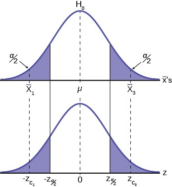
In Figure 9.3 two of the three possible outcomes are presented. X– 1 and X– 3 are in the tails of the hypothesized distribution of H0. Notice that the horizontal axis in the top panel is labeled X– ‘s. This is the same theoretical distribution of X– ‘s, the sampling distribution, that the Central Limit Theorem tells us is normally distributed. This is why we can draw it

with this shape. The horizontal axis of the bottom panel is labeled Z and is the standard normal distribution. Zα

2

and -Z α ,

2

called the critical values, are marked on the bottom panel as the Z values associated with the probability the analyst has set as the level of significance in the test, (α). The probabilities in the tails of both panels are, therefore, the same.

Notice that for each X– there is an associated Zc, called the calculated Z, that comes from solving the equation above. This calculated Z is nothing more than the number of standard deviations that the hypothesized mean is from the sample mean.

If the sample mean falls “too many” standard deviations from the hypothesized mean we conclude that the sample mean could not have come from the distribution with the hypothesized mean, given our pre-set required level of significance. It could have come from H0, but it is deemed just too unlikely. In Figure 9.3 both X 1 and X 3 are in the tails of the distribution. They are deemed “too far” from the hypothesized value of the mean given the chosen level of alpha. If in fact this sample mean it did come from H0, but from in the tail, we have made a Type I error: we have rejected a good null. Our

only real comfort is that we know the probability of making such an error, α, and we can control the size of α.

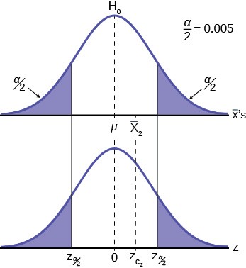
Figure 9.4 shows the third possibility for the location of the sample mean, x . Here the sample mean is within the two critical values. That is, within the probability of (1-α) and we cannot reject the null hypothesis.

Figure 9.4

This gives us the decision rule for testing a hypothesis for a two-tailed test:

Table 9.3

This rule will always be the same no matter what hypothesis we are testing or what formulas we are using to make the test. The only change will be to change the Zc to the appropriate symbol for the test statistic for the parameter being

This OpenStax book is available for free at http://cnx.org/content/col11776/1.33

tested. Stating the decision rule another way: if the sample mean is unlikely to have come from the distribution with the hypothesized mean we cannot accept the null hypothesis. Here we define “unlikely” as having a probability less than alpha of occurring.

P-Value Approach

An alternative decision rule can be developed by calculating the probability that a sample mean could be found that would give a test statistic larger than the test statistic found from the current sample data assuming that the null hypothesis is true. Here the notion of “likely” and “unlikely” is defined by the probability of drawing a sample with a mean from a population with the hypothesized mean that is either larger or smaller than that found in the sample data. Simply stated, the p-value approach compares the desired significance level, α, to the p-value which is the probability of drawing a sample mean further from the hypothesized value than the actual sample mean. A large p-value calculated from the data indicates that we should not reject the null hypothesis. The smaller the p-value, the more unlikely the outcome, and the stronger the evidence is against the null hypothesis. We would reject the null hypothesis if the evidence is strongly against it. The relationship between the decision rule of comparing the calculated test statistics, Zc, and the Critical Value, Zα , and using the p-value

can be seen in Figure 9.5.

Figure 9.5

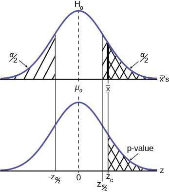
The calculated value of the test statistic is Zc in this example and is marked on the bottom graph of the standard normal distribution because it is a Z value. In this case the calculated value is in the tail and thus we cannot accept the null

hypothesis, the associated X– is just too unusually large to believe that it came from the distribution with a mean of µ0 with

a significance level of α.

If we use the p-value decision rule we need one more step. We need to find in the standard normal table the probability associated with the calculated test statistic, Zc. We then compare that to the α associated with our selected level of confidence. In Figure 9.5 we see that the p-value is less than α and therefore we cannot accept the null. We know that the p-value is less than α because the area under the p-value is smaller than α/2. It is important to note that two researchers drawing randomly from the same population may find two different P-values from their samples. This occurs because the

• value is calculated as the probability in the tail beyond the sample mean assuming that the null hypothesis is correct. Because the sample means will in all likelihood be different this will create two different P-values. Nevertheless, the conclusions as to the null hypothesis should be different with only the level of probability of α.

Here is a systematic way to make a decision of whether you cannot accept or cannot reject a null hypothesis if using the p-value and a preset or preconceived α (the ” significance level“). A preset α is the probability of a Type I error (rejecting the null hypothesis when the null hypothesis is true). It may or may not be given to you at the beginning of the problem. In any case, the value of α is the decision of the analyst. When you make a decision to reject or not reject H0, do as follows:

• If α > p-value, cannot accept H0. The results of the sample data are significant. There is sufficient evidence to conclude that H0 is an incorrect belief and that the alternative hypothesis, Ha, may be correct.
• If α ≤ p-value, cannot reject H0. The results of the sample data are not significant. There is not sufficient evidence to conclude that the alternative hypothesis, Ha, may be correct. In this case the status quo stands.
• When you “cannot reject H0“, it does not mean that you should believe that H0 is true. It simply means that the sample data have failed to provide sufficient evidence to cast serious doubt about the truthfulness of H0. Remember that the null is the status quo and it takes high probability to overthrow the status quo. This bias in favor of the null hypothesis is what gives rise to the statement “tyranny of the status quo” when discussing hypothesis testing and the scientific method.

Both decision rules will result in the same decision and it is a matter of preference which one is used.

One and Two-tailed Tests

The discussion of Figure 9.3–Figure 9.5 was based on the null and alternative hypothesis presented in Figure 9.3. This was called a two-tailed test because the alternative hypothesis allowed that the mean could have come from a population which was either larger or smaller than the hypothesized mean in the null hypothesis. This could be seen by the statement of the alternative hypothesis as μ ≠ 100, in this example.

It may be that the analyst has no concern about the value being “too” high or “too” low from the hypothesized value. If this is the case, it becomes a one-tailed test and all of the alpha probability is placed in just one tail and not split into α/2 as in the above case of a two-tailed test. Any test of a claim will be a one-tailed test. For example, a car manufacturer claims that their Model 17B provides gas mileage of greater than 25 miles per gallon. The null and alternative hypothesis would be:

H0: µ ≤ 25

Ha: µ > 25

The claim would be in the alternative hypothesis. The burden of proof in hypothesis testing is carried in the alternative. This is because failing to reject the null, the status quo, must be accomplished with 90 or 95 percent significance that it cannot be maintained. Said another way, we want to have only a 5 or 10 percent probability of making a Type I error, rejecting a good null; overthrowing the status quo.

This is a one-tailed test and all of the alpha probability is placed in just one tail and not split into α/2 as in the above case of a two-tailed test.

Figure 9.6 shows the two possible cases and the form of the null and alternative hypothesis that give rise to them.

This OpenStax book is available for free at http://cnx.org/content/col11776/1.33

Figure 9.6

where μ0 is the hypothesized value of the population mean.

Table 9.4 Test Statistics for Test of Means, Varying Sample Size, Population Standard Deviation Known or Unknown

Effects of Sample Size on Test Statistic

In developing the confidence intervals for the mean from a sample, we found that most often we would not have the population standard deviation, σ. If the sample size were larger than 30, we could simply substitute the point estimate for σ, the sample standard deviation, s, and use the student’s t distribution to correct for this lack of information.

When testing hypotheses we are faced with this same problem and the solution is exactly the same. Namely: If the population standard deviation is unknown, and the sample size is less than 30, substitute s, the point estimate for the population standard deviation, σ, in the formula for the test statistic and use the student’s t distribution. All the formulas and

figures above are unchanged except for this substitution and changing the Z distribution to the student’s t distribution on the graph. Remember that the student’s t distribution can only be computed knowing the proper degrees of freedom for the problem. In this case, the degrees of freedom is computed as before with confidence intervals: df = (n-1). The calculated t-value is compared to the t-value associated with the pre-set level of confidence required in the test, tα, df found in the student’s t tables. If we do not know σ, but the sample size is 30 or more, we simply substitute s for σ and use the normal distribution.

Table 9.4 summarizes these rules.

A Systematic Approach for Testing A Hypothesis

A systematic approach to hypothesis testing follows the following steps and in this order. This template will work for all hypotheses that you will ever test.

• Set up the null and alternative hypothesis. This is typically the hardest part of the process. Here the question being asked is reviewed. What parameter is being tested, a mean, a proportion, differences in means, etc. Is this a one-tailed test or two-tailed test? Remember, if someone is making a claim it will always be a one-tailed test.
• Decide the level of significance required for this particular case and determine the critical value. These can be found in the appropriate statistical table. The levels of confidence typical for the social sciences are 90, 95 and 99. However, the level of significance is a policy decision and should be based upon the risk of making a Type I error, rejecting a good null. Consider the consequences of making a Type I error.

Next, on the basis of the hypotheses and sample size, select the appropriate test statistic and find the relevant critical value: Zα, tα, etc. Drawing the relevant probability distribution and marking the critical value is always big help. Be sure to match the graph with the hypothesis, especially if it is a one-tailed test.

• Take a sample(s) and calculate the relevant parameters: sample mean, standard deviation, or proportion. Using the formula for the test statistic from above in step 2, now calculate the test statistic for this particular case using the parameters you have just calculated.
• Compare the calculated test statistic and the critical value. Marking these on the graph will give a good visual picture of the situation. There are now only two situations:
• The test statistic is in the tail: Cannot Accept the null, the probability that this sample mean (proportion) came from the hypothesized distribution is too small to believe that it is the real home of these sample data.
• The test statistic is not in the tail: Cannot Reject the null, the sample data are compatible with the hypothesized population parameter.
• Reach a conclusion. It is best to articulate the conclusion two different ways. First a formal statistical conclusion such as “With a 95 % level of significance we cannot accept the null hypotheses that the population mean is equal to XX (units of measurement)”. The second statement of the conclusion is less formal and states the action, or lack of action, required. If the formal conclusion was that above, then the informal one might be, “The machine is broken and we need to shut it down and call for repairs”.

All hypotheses tested will go through this same process. The only changes are the relevant formulas and those are determined by the hypothesis required to answer the original question.

| Full Hypothesis Test Examples

Tests on Means

Example 9.8Jeffrey, as an eight-year old, established a mean time of 16.43 seconds for swimming the 25-yard freestyle, with a standard deviation of 0.8 seconds. His dad, Frank, thought that Jeffrey could swim the 25-yard freestyle faster using goggles. Frank bought Jeffrey a new pair of expensive goggles and timed Jeffrey for 15 25-yard freestyle swims. For the 15 swims, Jeffrey’s mean time was 16 seconds. Frank thought that the goggles helped Jeffrey to swim faster than the 16.43 seconds. Conduct a hypothesis test using a preset α = 0.05.Solution 9.8Set up the Hypothesis Test:

This OpenStax book is available for free at http://cnx.org/content/col11776/1.33

Since the problem is about a mean, this is a test of a single population mean. Set the null and alternative hypothesis:

In this case there is an implied challenge or claim. This is that the goggles will reduce the swimming time. The effect of this is to set the hypothesis as a one-tailed test. The claim will always be in the alternative hypothesis because the burden of proof always lies with the alternative. Remember that the status quo must be defeated with a high degree of confidence, in this case 95 % confidence. The null and alternative hypotheses are thus:

H0: μ ≥ 16.43 Ha: μ < 16.43

For Jeffrey to swim faster, his time will be less than 16.43 seconds. The “<” tells you this is left-tailed. Determine the distribution needed:

Random variable: X¯ = the mean time to swim the 25-yard freestyle.

Distribution for the test statistic:

The sample size is less than 30 and we do not know the population standard deviation so this is a t-test. and the

X– – µ 0

proper formula is: tc = σ / n

μ0 = 16.43 comes from H0 and not the data. X– = 16. s = 0.8, and n = 15.

Our step 2, setting the level of significance, has already been determined by the problem, .05 for a 95 % significance level. It is worth thinking about the meaning of this choice. The Type I error is to conclude that Jeffrey swims the 25-yard freestyle, on average, in less than 16.43 seconds when, in fact, he actually swims the 25-yard freestyle, on average, in 16.43 seconds. (Reject the null hypothesis when the null hypothesis is true.) For this case the only concern with a Type I error would seem to be that Jeffery’s dad may fail to bet on his son’s victory because he does not have appropriate confidence in the effect of the goggles.

To find the critical value we need to select the appropriate test statistic. We have concluded that this is a t-test on the basis of the sample size and that we are interested in a population mean. We can now draw the graph of the t-distribution and mark the critical value. For this problem the degrees of freedom are n-1, or 14. Looking up 14 degrees of freedom at the 0.05 column of the t-table we find 1.761. This is the critical value and we can put this on our graph.

Step 3 is the calculation of the test statistic using the formula we have selected. We find that the calculated test statistic is 2.08, meaning that the sample mean is 2.08 standard deviations away from the hypothesized mean of 16.43.

t = x– – µ 0 = 16 – 16.43 = -2.08

cs

n

.8

15

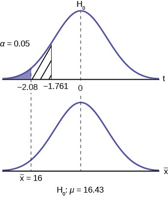
Figure 9.7

Step 4 has us compare the test statistic and the critical value and mark these on the graph. We see that the test statistic is in the tail and thus we move to step 4 and reach a conclusion. The probability that an average time of 16 minutes could come from a distribution with a population mean of 16.43 minutes is too unlikely for us to accept the null hypothesis. We cannot accept the null.

Step 5 has us state our conclusions first formally and then less formally. A formal conclusion would be stated as: “With a 95% level of significance we cannot accept the null hypothesis that the swimming time with goggles comes from a distribution with a population mean time of 16.43 minutes.” Less formally, “With 95% significance we believe that the goggles improves swimming speed”

9.8 The mean throwing distance of a football for Marco, a high school freshman quarterback, is 40 yards, with a standard deviation of two yards. The team coach tells Marco to adjust his grip to get more distance. The coach records the distances for 20 throws. For the 20 throws, Marco’s mean distance was 45 yards. The coach thought the different grip helped Marco throw farther than 40 yards. Conduct a hypothesis test using a preset α = 0.05. Assume the throw
If we wished to use the p-value system of reaching a conclusion we would calculate the statistic and take the additional step to find the probability of being 2.08 standard deviations from the mean on a t-distribution. This value is .0187. Comparing this to the α-level of .05 we see that we cannot accept the null. The p-value has been put on the graph as the shaded area beyond -2.08 and it shows that it is smaller than the hatched area which is the alpha level of 0.05. Both methods reach the same conclusion that we cannot accept the null hypothesis.

This OpenStax book is available for free at http://cnx.org/content/col11776/1.33

distances for footballs are normal.First, determine what type of test this is, set up the hypothesis test, find the p-value, sketch the graph, and state your conclusion.

Example 9.9

Jane has just begun her new job as on the sales force of a very competitive company. In a sample of 16 sales calls it was found that she closed the contract for an average value of 108 dollars with a standard deviation of 12 dollars. Test at 5% significance that the population mean is at least 100 dollars against the alternative that it is less than 100 dollars. Company policy requires that new members of the sales force must exceed an average of

$100 per contract during the trial employment period. Can we conclude that Jane has met this requirement at the significance level of 95%?

Solution 9.9

1. H0: µ ≤ 100 Ha: µ > 100

The null and alternative hypothesis are for the parameter µ because the number of dollars of the contracts is a continuous random variable. Also, this is a one-tailed test because the company has only an interested if the number of dollars per contact is below a particular number not “too high” a number. This can be thought of as making a claim that the requirement is being met and thus the claim is in the alternative hypothesis.

• Test statistic: t

= x¯ − µ0 = 108⎛ − 1⎞00 = 2.67

⎝⎠
cs

n

12 16

• Critical value: ta = 1.753 with n-1 degrees of freedom= 15

The test statistic is a Student’s t because the sample size is below 30; therefore, we cannot use the normal distribution. Comparing the calculated value of the test statistic and the critical value of t (ta) at a 5% significance level, we see that the calculated value is in the tail of the distribution. Thus, we conclude that 108

dollars per contract is significantly larger than the hypothesized value of 100 and thus we cannot accept the null hypothesis. There is evidence that supports Jane’s performance meets company standards.

Figure 9.8

9.9 It is believed that a stock price for a particular company will grow at a rate of $5 per week with a standard deviation of $1. An investor believes the stock won’t grow as quickly. The changes in stock price is recorded for ten weeks and are as follows: $4, $3, $2, $3, $1, $7, $2, $1, $1, $2. Perform a hypothesis test using a 5% level of significance. State the null and alternative hypotheses, state your conclusion, and identify the Type I errors.

Example 9.10

A manufacturer of salad dressings uses machines to dispense liquid ingredients into bottles that move along a filling line. The machine that dispenses salad dressings is working properly when 8 ounces are dispensed. Suppose that the average amount dispensed in a particular sample of 35 bottles is 7.91 ounces with a variance of

0.03 ounces squared, s2 . Is there evidence that the machine should be stopped and production wait for repairs?

The lost production from a shutdown is potentially so great that management feels that the level of significance in the analysis should be 99%.

Again we will follow the steps in our analysis of this problem.

Solution 9.10

STEP 1: Set the Null and Alternative Hypothesis. The random variable is the quantity of fluid placed in the bottles. This is a continuous random variable and the parameter we are interested in is the mean. Our hypothesis therefore is about the mean. In this case we are concerned that the machine is not filling properly. From what we are told it does not matter if the machine is over-filling or under-filling, both seem to be an equally bad error. This tells us that this is a two-tailed test: if the machine is malfunctioning it will be shutdown regardless if it is from over-filling or under-filling. The null and alternative hypotheses are thus:

H0 : µ = 8

Ha : µ ≠ 8

STEP 2: Decide the level of significance and draw the graph showing the critical value.

This problem has already set the level of significance at 99%. The decision seems an appropriate one and shows the thought process when setting the significance level. Management wants to be very certain, as certain as probability will allow, that they are not shutting down a machine that is not in need of repair. To draw the distribution and the critical value, we need to know which distribution to use. Because this is a continuous random variable and we are interested in the mean, and the sample size is greater than 30, the appropriate distribution is the normal distribution and the relevant critical value is 2.575 from the normal table or the t-table at 0.005 column and infinite degrees of freedom. We draw the graph and mark these points.

This OpenStax book is available for free at http://cnx.org/content/col11776/1.33

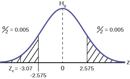
Figure 9.9

STEP 3: Calculate sample parameters and the test statistic. The sample parameters are provided, the sample mean is 7.91 and the sample variance is .03 and the sample size is 35. We need to note that the sample variance was provided not the sample standard deviation, which is what we need for the formula. Remembering that the standard deviation is simply the square root of the variance, we therefore know the sample standard deviation, s, is 0.173. With this information we calculate the test statistic as -3.07, and mark it on the graph.

Z = x– – µ 0 = 7.91 – 8 = -3.07

cs

n

.173

35

STEP 4: Compare test statistic and the critical values Now we compare the test statistic and the critical value by placing the test statistic on the graph. We see that the test statistic is in the tail, decidedly greater than the critical value of 2.575. We note that even the very small difference between the hypothesized value and the sample value is still a large number of standard deviations. The sample mean is only 0.08 ounces different from the required level of 8 ounces, but it is 3 plus standard deviations away and thus we cannot accept the null hypothesis.

STEP 5: Reach a Conclusion

Three standard deviations of a test statistic will guarantee that the test will fail. The probability that anything is within three standard deviations is almost zero. Actually it is 0.0026 on the normal distribution, which is certainly almost zero in a practical sense. Our formal conclusion would be “ At a 99% level of significance we cannot accept the hypothesis that the sample mean came from a distribution with a mean of 8 ounces” Or less formally, and getting to the point, “At a 99% level of significance we conclude that the machine is under filling the bottles and is in need of repair”.

Hypothesis Test for Proportions

Just as there were confidence intervals for proportions, or more formally, the population parameter p of the binomial distribution, there is the ability to test hypotheses concerning p.

The population parameter for the binomial is p. The estimated value (point estimate) for p is p′ where p′ = x/n, x is the number of successes in the sample and n is the sample size.

When you perform a hypothesis test of a population proportion p, you take a simple random sample from the population. The conditions for a binomial distribution must be met, which are: there are a certain number n of independent trials meaning random sampling, the outcomes of any trial are binary, success or failure, and each trial has the same probability of a success p. The shape of the binomial distribution needs to be similar to the shape of the normal distribution. To ensure

this, the quantities np′ and nq′ must both be greater than five (np′ > 5 and nq′ > 5). In this case the binomial distribution of a sample (estimated) proportion can be approximated by the normal distribution with µ = np and σ = npq . Remember that q = 1 – p . There is no distribution that can correct for this small sample bias and thus if these conditions are not

met we simply cannot test the hypothesis with the data available at that time. We met this condition when we first were estimating confidence intervals for p.

Again, we begin with the standardizing formula modified because this is the distribution of a binomial.

Z =
p’ – p pq n

p’ – p0p0 q0n
Substituting p0 , the hypothesized value of p, we have:

Zc =

This is the test statistic for testing hypothesized values of p, where the null and alternative hypotheses take one of the following forms:

Table 9.5

The decision rule stated above applies here also: if the calculated value of Zc shows that the sample proportion is “too many” standard deviations from the hypothesized proportion, the null hypothesis cannot be accepted. The decision as to what is “too many” is pre-determined by the analyst depending on the level of significance required in the test.

Example 9.11The mortgage department of a large bank is interested in the nature of loans of first-time borrowers. This information will be used to tailor their marketing strategy. They believe that 50% of first-time borrowers take out smaller loans than other borrowers. They perform a hypothesis test to determine if the percentage is the same or different from 50%. They sample 100 first-time borrowers and find 53 of these loans are smaller that the other borrowers. For the hypothesis test, they choose a 5% level of significance.Solution 9.11STEP 1: Set the null and alternative hypothesis.H0: p = 0.50 Ha: p ≠ 0.50The words “is the same or different from” tell you this is a two-tailed test. The Type I and Type II errors are as follows: The Type I error is to conclude that the proportion of borrowers is different from 50% when, in fact, the proportion is actually 50%. (Reject the null hypothesis when the null hypothesis is true). The Type II error is there is not enough evidence to conclude that the proportion of first time borrowers differs from 50% when, in fact, the proportion does differ from 50%. (You fail to reject the null hypothesis when the null hypothesis is false.)STEP 2: Decide the level of significance and draw the graph showing the critical valueThe level of significance has been set by the problem at the 95% level. Because this is two-tailed test one-half of the alpha value will be in the upper tail and one-half in the lower tail as shown on the graph. The critical value for the normal distribution at the 95% level of confidence is 1.96. This can easily be found on the student’s t- table at the very bottom at infinite degrees of freedom remembering that at infinity the t-distribution is the normal distribution. Of course the value can also be found on the normal table but you have go looking for one-half of 95 (0.475) inside the body of the table and then read out to the sides and top for the number of standard deviations.

This OpenStax book is available for free at http://cnx.org/content/col11776/1.33

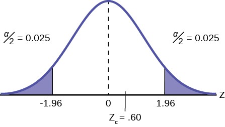
Figure 9.10

STEP 3: Calculate the sample parameters and critical value of the test statistic. The test statistic is a normal distribution, Z, for testing proportions and is:

p’ – p0p0 q0n

== 0.60
=
Z.53 – .50

.5(.5)

100

For this case, the sample of 100 found 53 first-time borrowers were different from other borrowers. The sample proportion, p′ = 53/100= 0.53 The test question, therefore, is : “Is 0.53 significantly different from .50?” Putting these values into the formula for the test statistic we find that 0.53 is only 0.60 standard deviations away from .50. This is barely off of the mean of the standard normal distribution of zero. There is virtually no difference from the sample proportion and the hypothesized proportion in terms of standard deviations.

STEP 4: Compare the test statistic and the critical value.

The calculated value is well within the critical values of ± 1.96 standard deviations and thus we cannot reject the null hypothesis. To reject the null hypothesis we need significant evident of difference between the hypothesized value and the sample value. In this case the sample value is very nearly the same as the hypothesized value measured in terms of standard deviations.

STEP 5: Reach a conclusion

The formal conclusion would be “At a 95% level of significance we cannot reject the null hypothesis that 50% of first-time borrowers have the same size loans as other borrowers”. Less formally we would say that “There is no evidence that one-half of first-time borrowers are significantly different in loan size from other borrowers”. Notice the length to which the conclusion goes to include all of the conditions that are attached to the conclusion. Statisticians for all the criticism they receive, are careful to be very specific even when this seems trivial. Statisticians cannot say more than they know and the data constrain the conclusion to be within the metes and bounds of the data.

9.11 A teacher believes that 85% of students in the class will want to go on a field trip to the local zoo. She performs a hypothesis test to determine if the percentage is the same or different from 85%. The teacher samples 50 students and 39 reply that they would want to go to the zoo. For the hypothesis test, use a 1% level of significance.

Example 9.12Suppose a consumer group suspects that the proportion of households that have three or more cell phones is 30%. A cell phone company has reason to believe that the proportion is not 30%. Before they start a big advertising campaign, they conduct a hypothesis test. Their marketing people survey 150 households with the result that 43 of the households have three or more cell phones.Solution 9.12Here is an abbreviate version of the system to solve hypothesis tests applied to a test on a proportions.H0 : p = 0.3Ha : p ≠ 0.3n = 150p’ = x = 43 = 0.287n150Zc = p’ – p0 = 0.287 – 0.3 = 0.347p0 q0n.3(.7)150Figure 9.11

Example 9.13The National Institute of Standards and Technology provides exact data on conductivity properties of materials. Following are conductivity measurements for 11 randomly selected pieces of a particular type of glass.1.11; 1.07; 1.11; 1.07; 1.12; 1.08; .98; .98 1.02; .95; .95Is there convincing evidence that the average conductivity of this type of glass is greater than one? Use a significance level of 0.05.Solution 9.13Let’s follow a four-step process to answer this statistical question.1. State the Question: We need to determine if, at a 0.05 significance level, the average conductivity of the

This OpenStax book is available for free at http://cnx.org/content/col11776/1.33

selected glass is greater than one. Our hypotheses will be a. H0: μ ≤ 1

• Ha: μ > 1
• Plan: We are testing a sample mean without a known population standard deviation with less than 30 observations. Therefore, we need to use a Student’s-t distribution. Assume the underlying population is normal.

Do the calculations and draw the graph.

• State the Conclusions: We cannot accept the null hypothesis. It is reasonable to state that the data supports the claim that the average conductivity level is greater than one.

Example 9.14In a study of 420,019 cell phone users, 172 of the subjects developed brain cancer. Test the claim that cell phone users developed brain cancer at a greater rate than that for non-cell phone users (the rate of brain cancer for non-cell phone users is 0.0340%). Since this is a critical issue, use a 0.005 significance level. Explain why the significance level should be so low in terms of a Type I error.Solution 9.14We need to conduct a hypothesis test on the claimed cancer rate. Our hypotheses will be a. H0: p ≤ 0.00034b. Ha: p > 0.00034If we commit a Type I error, we are essentially accepting a false claim. Since the claim describes cancer- causing environments, we want to minimize the chances of incorrectly identifying causes of cancer.We will be testing a sample proportion with x = 172 and n = 420,019. The sample is sufficiently large because we have np’ = 420,019(0.00034) = 142.8, nq’ = 420,019(0.99966) = 419,876.2, two independent outcomes, and a fixed probability of success p’ = 0.00034. Thus we will be able to generalize our results to the population.

KEY TERMS

Binomial Distribution a discrete random variable (RV) that arises from Bernoulli trials. There are a fixed number, n, of independent trials. “Independent” means that the result of any trial (for example, trial 1) does not affect the results of the following trials, and all trials are conducted under the same conditions. Under these circumstances the binomial RV Χ is defined as the number of successes in n trials. The notation is: X ~ B(n, p) μ = np and the standard

⎝x⎠
deviation is σ =npq . The probability of exactly x successes in n trials is P(X = x) = ⎛n⎞px qn − x .

Central Limit Theorem Given a random variable (RV) with known mean µ and known standard deviation σ. We are

sampling with size n and we are interested in two new RVs – the sample mean, X¯ . If the size n of the sample is sufficiently large, then X¯ ~ N⎛µ, σ ⎞ . If the size n of the sample is sufficiently large, then the distribution of the

⎝n⎠

sample means will approximate a normal distribution regardless of the shape of the population. The expected value

of the mean of the sample means will equal the population mean. The standard deviation of the distribution of the

n
sample means, σ , is called the standard error of the mean.

Confidence Interval (CI) an interval estimate for an unknown population parameter. This depends on:

• The desired confidence level.
• Information that is known about the distribution (for example, known standard deviation).
• The sample and its size.

Critical Value The t or Z value set by the researcher that measures the probability of a Type I error, α.

Hypothesis a statement about the value of a population parameter, in case of two hypotheses, the statement assumed to be true is called the null hypothesis (notation H0) and the contradictory statement is called the alternative hypothesis (notation Ha).

Hypothesis Testing Based on sample evidence, a procedure for determining whether the hypothesis stated is a reasonable statement and should not be rejected, or is unreasonable and should be rejected.

Normal Distribution

a continuous random variable (RV) with pdf f (x) =1 e

σ 2π

−(x − µ)2

2σ 2, where μ is the mean of

the distribution, and σ is the standard deviation, notation: X ~ N(μ, σ). If μ = 0 and σ = 1, the RV is called the standard normal distribution.

Standard Deviation a number that is equal to the square root of the variance and measures how far data values are from their mean; notation: s for sample standard deviation and σ for population standard deviation.

Student’s t-Distribution investigated and reported by William S. Gossett in 1908 and published under the pseudonym Student. The major characteristics of the random variable (RV) are:

• It is continuous and assumes any real values.
• The pdf is symmetrical about its mean of zero. However, it is more spread out and flatter at the apex than the normal distribution.
• It approaches the standard normal distribution as n gets larger.
• There is a “family” of t distributions: every representative of the family is completely defined by the number of degrees of freedom which is one less than the number of data items.

Test Statistic The formula that counts the number of standard deviations on the relevant distribution that estimated parameter is away from the hypothesized value.

Type I Error The decision is to reject the null hypothesis when, in fact, the null hypothesis is true.

Type II Error The decision is not to reject the null hypothesis when, in fact, the null hypothesis is false.

This OpenStax book is available for free at http://cnx.org/content/col11776/1.33

CHAPTER REVIEW

Null and Alternative Hypotheses

In a hypothesis test, sample data is evaluated in order to arrive at a decision about some type of claim. If certain conditions about the sample are satisfied, then the claim can be evaluated for a population. In a hypothesis test, we:

• Evaluate the null hypothesis, typically denoted with H0. The null is not rejected unless the hypothesis test shows otherwise. The null statement must always contain some form of equality (=, ≤ or ≥)
• Always write the alternative hypothesis, typically denoted with Ha or H1, using not equal, less than or greater than symbols, i.e., (≠, <, or > ).
• If we reject the null hypothesis, then we can assume there is enough evidence to support the alternative hypothesis.
• Never state that a claim is proven true or false. Keep in mind the underlying fact that hypothesis testing is based on probability laws; therefore, we can talk only in terms of non-absolute certainties.

Outcomes and the Type I and Type II Errors

In every hypothesis test, the outcomes are dependent on a correct interpretation of the data. Incorrect calculations or misunderstood summary statistics can yield errors that affect the results. A Type I error occurs when a true null hypothesis is rejected. A Type II error occurs when a false null hypothesis is not rejected.

The probabilities of these errors are denoted by the Greek letters α and β, for a Type I and a Type II error respectively. The power of the test, 1 – β, quantifies the likelihood that a test will yield the correct result of a true alternative hypothesis being accepted. A high power is desirable.

Distribution Needed for Hypothesis Testing

In order for a hypothesis test’s results to be generalized to a population, certain requirements must be satisfied. When testing for a single population mean:

• A Student’s t-test should be used if the data come from a simple, random sample and the population is approximately normally distributed, or the sample size is large, with an unknown standard deviation.
• The normal test will work if the data come from a simple, random sample and the population is approximately normally distributed, or the sample size is large.

When testing a single population proportion use a normal test for a single population proportion if the data comes from a simple, random sample, fill the requirements for a binomial distribution, and the mean number of success and the mean number of failures satisfy the conditions: np > 5 and nq > n where n is the sample size, p is the probability of a success, and q is the probability of a failure.

Full Hypothesis Test Examples

The hypothesis test itself has an established process. This can be summarized as follows:

• Determine H0 and Ha. Remember, they are contradictory.
• Determine the random variable.
• Determine the distribution for the test.
• Draw a graph and calculate the test statistic.
• Compare the calculated test statistic with the Z critical value determined by the level of significance required by the test and make a decision (cannot reject H0 or cannot accept H0), and write a clear conclusion using English sentences.

FORMULA REVIEW

Sample SizeTest Statistic> 30(σ unknown)X– – µ 0Zc = s /n> 30(σ known)X– – µ 0Zc = σ /n
9.3 Distribution Needed for Hypothesis Testing

Sample SizeTest Statistic< 30(σ unknown)X– – µ 0tc = s /n< 30(σ known)X– – µ 0Zc = σ /n
Table 9.6 Test Statistics for Test of Means, Varying Sample Size, Population Known or Unknown

Table 9.6 Test Statistics for Test of Means, Varying Sample Size, Population Known or Unknown

PRACTICE

• Null and Alternative Hypotheses
• You are testing that the mean speed of your cable Internet connection is more than three Megabits per second. What is the random variable? Describe in words.
• You are testing that the mean speed of your cable Internet connection is more than three Megabits per second. State the null and alternative hypotheses.
• The American family has an average of two children. What is the random variable? Describe in words.
• The mean entry level salary of an employee at a company is $58,000. You believe it is higher for IT professionals in the company. State the null and alternative hypotheses.
• A sociologist claims the probability that a person picked at random in Times Square in New York City is visiting the area is 0.83. You want to test to see if the proportion is actually less. What is the random variable? Describe in words.
• A sociologist claims the probability that a person picked at random in Times Square in New York City is visiting the area is 0.83. You want to test to see if the claim is correct. State the null and alternative hypotheses.
• In a population of fish, approximately 42% are female. A test is conducted to see if, in fact, the proportion is less. State the null and alternative hypotheses.
• Suppose that a recent article stated that the mean time spent in jail by a first–time convicted burglar is 2.5 years. A study was then done to see if the mean time has increased in the new century. A random sample of 26 first-time convicted burglars in a recent year was picked. The mean length of time in jail from the survey was 3 years with a standard deviation of 1.8 years. Suppose that it is somehow known that the population standard deviation is 1.5. If you were conducting a hypothesis test to determine if the mean length of jail time has increased, what would the null and alternative hypotheses be? The distribution of the population is normal.
• H0:
• Ha:
• A random survey of 75 death row inmates revealed that the mean length of time on death row is 17.4 years with a standard deviation of 6.3 years. If you were conducting a hypothesis test to determine if the population mean time on death row could likely be 15 years, what would the null and alternative hypotheses be?
• H0:
• Ha:
• The National Institute of Mental Health published an article stating that in any one-year period, approximately 9.5 percent of American adults suffer from depression or a depressive illness. Suppose that in a survey of 100 people in a certain town, seven of them suffered from depression or a depressive illness. If you were conducting a hypothesis test to determine if the true proportion of people in that town suffering from depression or a depressive illness is lower than the percent in the general adult American population, what would the null and alternative hypotheses be?
• H0:
• Ha:

This OpenStax book is available for free at http://cnx.org/content/col11776/1.33

Outcomes and the Type I and Type II Errors

• The mean price of mid-sized cars in a region is $32,000. A test is conducted to see if the claim is true. State the Type I and Type II errors in complete sentences.
• A sleeping bag is tested to withstand temperatures of –15 °F. You think the bag cannot stand temperatures that low. State the Type I and Type II errors in complete sentences.
• For Exercise 9.12, what are α and β in words?
• In words, describe 1 – β For Exercise 9.12.
• A group of doctors is deciding whether or not to perform an operation. Suppose the null hypothesis, H0, is: the surgical procedure will go well. State the Type I and Type II errors in complete sentences.
• A group of doctors is deciding whether or not to perform an operation. Suppose the null hypothesis, H0, is: the surgical procedure will go well. Which is the error with the greater consequence?
• The power of a test is 0.981. What is the probability of a Type II error?
• A group of divers is exploring an old sunken ship. Suppose the null hypothesis, H0, is: the sunken ship does not contain buried treasure. State the Type I and Type II errors in complete sentences.
• A microbiologist is testing a water sample for E-coli. Suppose the null hypothesis, H0, is: the sample does not contain E- coli. The probability that the sample does not contain E-coli, but the microbiologist thinks it does is 0.012. The probability that the sample does contain E-coli, but the microbiologist thinks it does not is 0.002. What is the power of this test?
• A microbiologist is testing a water sample for E-coli. Suppose the null hypothesis, H0, is: the sample contains E-coli. Which is the error with the greater consequence?

Distribution Needed for Hypothesis Testing

• Which two distributions can you use for hypothesis testing for this chapter?
• Which distribution do you use when you are testing a population mean and the population standard deviation is known? Assume sample size is large. Assume a normal distribution with n ≥ 30.
• Which distribution do you use when the standard deviation is not known and you are testing one population mean? Assume a normal distribution, with n ≥ 30.
• A population mean is 13. The sample mean is 12.8, and the sample standard deviation is two. The sample size is 20. What distribution should you use to perform a hypothesis test? Assume the underlying population is normal.
• A population has a mean is 25 and a standard deviation of five. The sample mean is 24, and the sample size is 108. What distribution should you use to perform a hypothesis test?
• It is thought that 42% of respondents in a taste test would prefer Brand A. In a particular test of 100 people, 39% preferred Brand A. What distribution should you use to perform a hypothesis test?
• You are performing a hypothesis test of a single population mean using a Student’s t-distribution. What must you assume about the distribution of the data?
• You are performing a hypothesis test of a single population mean using a Student’s t-distribution. The data are not from a simple random sample. Can you accurately perform the hypothesis test?
• You are performing a hypothesis test of a single population proportion. What must be true about the quantities of np

and nq?

• You are performing a hypothesis test of a single population proportion. You find out that np is less than five. What must you do to be able to perform a valid hypothesis test?
• You are performing a hypothesis test of a single population proportion. The data come from which distribution?

Full Hypothesis Test Examples

• Assume H0: μ = 9 and Ha: μ < 9. Is this a left-tailed, right-tailed, or two-tailed test?
• Assume H0: μ ≤ 6 and Ha: μ > 6. Is this a left-tailed, right-tailed, or two-tailed test?
• Assume H0: p = 0.25 and Ha: p ≠ 0.25. Is this a left-tailed, right-tailed, or two-tailed test?

• Draw the general graph of a left-tailed test.
• Draw the graph of a two-tailed test.
• A bottle of water is labeled as containing 16 fluid ounces of water. You believe it is less than that. What type of test would you use?
• Your friend claims that his mean golf score is 63. You want to show that it is higher than that. What type of test would you use?
• A bathroom scale claims to be able to identify correctly any weight within a pound. You think that it cannot be that accurate. What type of test would you use?
• You flip a coin and record whether it shows heads or tails. You know the probability of getting heads is 50%, but you think it is less for this particular coin. What type of test would you use?
• If the alternative hypothesis has a not equals ( ≠ ) symbol, you know to use which type of test?
• Assume the null hypothesis states that the mean is at least 18. Is this a left-tailed, right-tailed, or two-tailed test?
• Assume the null hypothesis states that the mean is at most 12. Is this a left-tailed, right-tailed, or two-tailed test?
• Assume the null hypothesis states that the mean is equal to 88. The alternative hypothesis states that the mean is not equal to 88. Is this a left-tailed, right-tailed, or two-tailed test?

HOMEWORK

Null and Alternative Hypotheses

• Some of the following statements refer to the null hypothesis, some to the alternate hypothesis.

State the null hypothesis, H0, and the alternative hypothesis. Ha, in terms of the appropriate parameter (μ or p).

• The mean number of years Americans work before retiring is 34.
• At most 60% of Americans vote in presidential elections.
• The mean starting salary for San Jose State University graduates is at least $100,000 per year.
• Twenty-nine percent of high school seniors get drunk each month.
• Fewer than 5% of adults ride the bus to work in Los Angeles.
• The mean number of cars a person owns in her lifetime is not more than ten.
• About half of Americans prefer to live away from cities, given the choice.
• Europeans have a mean paid vacation each year of six weeks.
• The chance of developing breast cancer is under 11% for women.
• Private universities’ mean tuition cost is more than $20,000 per year.
• Over the past few decades, public health officials have examined the link between weight concerns and teen girls’ smoking. Researchers surveyed a group of 273 randomly selected teen girls living in Massachusetts (between 12 and 15 years old). After four years the girls were surveyed again. Sixty-three said they smoked to stay thin. Is there good evidence that more than thirty percent of the teen girls smoke to stay thin? The alternative hypothesis is:

a. p < 0.30

b. p ≤ 0.30 c. p ≥ 0.30 d. p > 0.30

• A statistics instructor believes that fewer than 20% of Evergreen Valley College (EVC) students attended the opening night midnight showing of the latest Harry Potter movie. She surveys 84 of her students and finds that 11 attended the midnight showing. An appropriate alternative hypothesis is:

a. p = 0.20 b. p > 0.20 c. p < 0.20

d. p ≤ 0.20

This OpenStax book is available for free at http://cnx.org/content/col11776/1.33

• Previously, an organization reported that teenagers spent 4.5 hours per week, on average, on the phone. The organization thinks that, currently, the mean is higher. Fifteen randomly chosen teenagers were asked how many hours per week they spend on the phone. The sample mean was 4.75 hours with a sample standard deviation of 2.0. Conduct a hypothesis test. The null and alternative hypotheses are:

a. Ho: x¯ = 4.5, Ha : x¯ > 4.5

b. Ho: μ ≥ 4.5, Ha: μ < 4.5

c. Ho: μ = 4.75, Ha: μ > 4.75 d. Ho: μ = 4.5, Ha: μ > 4.5

Outcomes and the Type I and Type II Errors

• State the Type I and Type II errors in complete sentences given the following statements.
• The mean number of years Americans work before retiring is 34.
• At most 60% of Americans vote in presidential elections.
• The mean starting salary for San Jose State University graduates is at least $100,000 per year.
• Twenty-nine percent of high school seniors get drunk each month.
• Fewer than 5% of adults ride the bus to work in Los Angeles.
• The mean number of cars a person owns in his or her lifetime is not more than ten.
• About half of Americans prefer to live away from cities, given the choice.
• Europeans have a mean paid vacation each year of six weeks.
• The chance of developing breast cancer is under 11% for women.
• Private universities mean tuition cost is more than $20,000 per year.
• For statements a-j in Exercise 9.109, answer the following in complete sentences.
• State a consequence of committing a Type I error.
• State a consequence of committing a Type II error.
• When a new drug is created, the pharmaceutical company must subject it to testing before receiving the necessary permission from the Food and Drug Administration (FDA) to market the drug. Suppose the null hypothesis is “the drug is unsafe.” What is the Type II Error?
• To conclude the drug is safe when in, fact, it is unsafe.
• Not to conclude the drug is safe when, in fact, it is safe.
• To conclude the drug is safe when, in fact, it is safe.
• Not to conclude the drug is unsafe when, in fact, it is unsafe.
• A statistics instructor believes that fewer than 20% of Evergreen Valley College (EVC) students attended the opening midnight showing of the latest Harry Potter movie. She surveys 84 of her students and finds that 11 of them attended the midnight showing. The Type I error is to conclude that the percent of EVC students who attended is .
• at least 20%, when in fact, it is less than 20%.
• 20%, when in fact, it is 20%.
• less than 20%, when in fact, it is at least 20%.
• less than 20%, when in fact, it is less than 20%.
• It is believed that Lake Tahoe Community College (LTCC) Intermediate Algebra students get less than seven hours of sleep per night, on average. A survey of 22 LTCC Intermediate Algebra students generated a mean of 7.24 hours with a standard deviation of 1.93 hours. At a level of significance of 5%, do LTCC Intermediate Algebra students get less than seven hours of sleep per night, on average?

The Type II error is not to reject that the mean number of hours of sleep LTCC students get per night is at least seven when, in fact, the mean number of hours

• is more than seven hours.
• is at most seven hours.
• is at least seven hours.
• is less than seven hours.

• Previously, an organization reported that teenagers spent 4.5 hours per week, on average, on the phone. The organization thinks that, currently, the mean is higher. Fifteen randomly chosen teenagers were asked how many hours per week they spend on the phone. The sample mean was 4.75 hours with a sample standard deviation of 2.0. Conduct a hypothesis test, the Type I error is:
• to conclude that the current mean hours per week is higher than 4.5, when in fact, it is higher
• to conclude that the current mean hours per week is higher than 4.5, when in fact, it is the same
• to conclude that the mean hours per week currently is 4.5, when in fact, it is higher
• to conclude that the mean hours per week currently is no higher than 4.5, when in fact, it is not higher

Distribution Needed for Hypothesis Testing

• It is believed that Lake Tahoe Community College (LTCC) Intermediate Algebra students get less than seven hours of sleep per night, on average. A survey of 22 LTCC Intermediate Algebra students generated a mean of 7.24 hours with a

standard deviation of 1.93 hours. At a level of significance of 5%, do LTCC Interme–diate Algebra students get less than

seven hours of sleep per night, on average? The distribution to be used for this test is X ~

a.N(7.24, 1.93)

22

b.N(7.24, 1.93)

• t22
• t21

Full Hypothesis Test Examples

• A particular brand of tires claims that its deluxe tire averages at least 50,000 miles before it needs to be replaced. From past studies of this tire, the standard deviation is known to be 8,000. A survey of owners of that tire design is conducted. From the 28 tires surveyed, the mean lifespan was 46,500 miles with a standard deviation of 9,800 miles. Using alpha = 0.05, is the data highly inconsistent with the claim?
• From generation to generation, the mean age when smokers first start to smoke varies. However, the standard deviation of that age remains constant of around 2.1 years. A survey of 40 smokers of this generation was done to see if the mean starting age is at least 19. The sample mean was 18.1 with a sample standard deviation of 1.3. Do the data support the claim at the 5% level?
• The cost of a daily newspaper varies from city to city. However, the variation among prices remains steady with a standard deviation of 20¢. A study was done to test the claim that the mean cost of a daily newspaper is $1.00. Twelve costs yield a mean cost of 95¢ with a standard deviation of 18¢. Do the data support the claim at the 1% level?
• An article in the San Jose Mercury News stated that students in the California state university system take 4.5 years, on average, to finish their undergraduate degrees. Suppose you believe that the mean time is longer. You conduct a survey of 49 students and obtain a sample mean of 5.1 with a sample standard deviation of 1.2. Do the data support your claim at the 1% level?
• The mean number of sick days an employee takes per year is believed to be about ten. Members of a personnel department do not believe this figure. They randomly survey eight employees. The number of sick days they took for the past year are as follows: 12; 4; 15; 3; 11; 8; 6; 8. Let x = the number of sick days they took for the past year. Should the personnel team believe that the mean number is ten?
• In 1955, Life Magazine reported that the 25 year-old mother of three worked, on average, an 80 hour week. Recently, many groups have been studying whether or not the women’s movement has, in fact, resulted in an increase in the average work week for women (combining employment and at-home work). Suppose a study was done to determine if the mean work week has increased. 81 women were surveyed with the following results. The sample mean was 83; the sample standard deviation was ten. Does it appear that the mean work week has increased for women at the 5% level?
• Your statistics instructor claims that 60 percent of the students who take her Elementary Statistics class go through life feeling more enriched. For some reason that she can’t quite figure out, most people don’t believe her. You decide to check this out on your own. You randomly survey 64 of her past Elementary Statistics students and find that 34 feel more enriched as a result of her class. Now, what do you think?
• A Nissan Motor Corporation advertisement read, “The average man’s I.Q. is 107. The average brown trout’s I.Q. is 4. So why can’t man catch brown trout?” Suppose you believe that the brown trout’s mean I.Q. is greater than four. You catch 12 brown trout. A fish psychologist determines the I.Q.s as follows: 5; 4; 7; 3; 6; 4; 5; 3; 6; 3; 8; 5. Conduct a hypothesis test of your belief.

This OpenStax book is available for free at http://cnx.org/content/col11776/1.33

• Refer to Exercise 9.119. Conduct a hypothesis test to see if your decision and conclusion would change if your belief were that the brown trout’s mean I.Q. is not four.
• According to an article in Newsweek, the natural ratio of girls to boys is 100:105. In China, the birth ratio is 100: 114 (46.7% girls). Suppose you don’t believe the reported figures of the percent of girls born in China. You conduct a study. In this study, you count the number of girls and boys born in 150 randomly chosen recent births. There are 60 girls and 90 boys born of the 150. Based on your study, do you believe that the percent of girls born in China is 46.7?
• A poll done for Newsweek found that 13% of Americans have seen or sensed the presence of an angel. A contingent doubts that the percent is really that high. It conducts its own survey. Out of 76 Americans surveyed, only two had seen or sensed the presence of an angel. As a result of the contingent’s survey, would you agree with the Newsweek poll? In complete sentences, also give three reasons why the two polls might give different results.
• The mean work week for engineers in a start-up company is believed to be about 60 hours. A newly hired engineer hopes that it’s shorter. She asks ten engineering friends in start-ups for the lengths of their mean work weeks. Based on the results that follow, should she count on the mean work week to be shorter than 60 hours?

Data (length of mean work week): 70; 45; 55; 60; 65; 55; 55; 60; 50; 55.

• Sixty-eight percent of online courses taught at community colleges nationwide were taught by full-time faculty. To test if 68% also represents California’s percent for full-time faculty teaching the online classes, Long Beach City College (LBCC) in California, was randomly selected for comparison. In the same year, 34 of the 44 online courses LBCC offered were taught by full-time faculty. Conduct a hypothesis test to determine if 68% represents California. NOTE: For more accurate results, use more California community colleges and this past year’s data.
• According to an article in Bloomberg Businessweek, New York City’s most recent adult smoking rate is 14%. Suppose that a survey is conducted to determine this year’s rate. Nine out of 70 randomly chosen N.Y. City residents reply that they smoke. Conduct a hypothesis test to determine if the rate is still 14% or if it has decreased.
• The mean age of De Anza College students in a previous term was 26.6 years old. An instructor thinks the mean age for online students is older than 26.6. She randomly surveys 56 online students and finds that the sample mean is 29.4 with a standard deviation of 2.1. Conduct a hypothesis test.
• Registered nurses earned an average annual salary of $69,110. For that same year, a survey was conducted of 41 California registered nurses to determine if the annual salary is higher than $69,110 for California nurses. The sample average was $71,121 with a sample standard deviation of $7,489. Conduct a hypothesis test.
• La Leche League International reports that the mean age of weaning a child from breastfeeding is age four to five worldwide. In America, most nursing mothers wean their children much earlier. Suppose a random survey is conducted of 21 U.S. mothers who recently weaned their children. The mean weaning age was nine months (3/4 year) with a standard deviation of 4 months. Conduct a hypothesis test to determine if the mean weaning age in the U.S. is less than four years old.
• Over the past few decades, public health officials have examined the link between weight concerns and teen girls’ smoking. Researchers surveyed a group of 273 randomly selected teen girls living in Massachusetts (between 12 and 15 years old). After four years the girls were surveyed again. Sixty-three said they smoked to stay thin. Is there good evidence that more than thirty percent of the teen girls smoke to stay thin?

After conducting the test, your decision and conclusion are

• Reject H0: There is sufficient evidence to conclude that more than 30% of teen girls smoke to stay thin.
• Do not reject H0: There is not sufficient evidence to conclude that less than 30% of teen girls smoke to stay thin.
• Do not reject H0: There is not sufficient evidence to conclude that more than 30% of teen girls smoke to stay thin.
• Reject H0: There is sufficient evidence to conclude that less than 30% of teen girls smoke to stay thin.

• A statistics instructor believes that fewer than 20% of Evergreen Valley College (EVC) students attended the opening night midnight showing of the latest Harry Potter movie. She surveys 84 of her students and finds that 11 of them attended the midnight showing.

At a 1% level of significance, an appropriate conclusion is:

• There is insufficient evidence to conclude that the percent of EVC students who attended the midnight showing of Harry Potter is less than 20%.
• There is sufficient evidence to conclude that the percent of EVC students who attended the midnight showing of Harry Potter is more than 20%.
• There is sufficient evidence to conclude that the percent of EVC students who attended the midnight showing of Harry Potter is less than 20%.
• There is insufficient evidence to conclude that the percent of EVC students who attended the midnight showing of Harry Potter is at least 20%.
• Previously, an organization reported that teenagers spent 4.5 hours per week, on average, on the phone. The organization thinks that, currently, the mean is higher. Fifteen randomly chosen teenagers were asked how many hours per week they spend on the phone. The sample mean was 4.75 hours with a sample standard deviation of 2.0. Conduct a hypothesis test.

At a significance level of a = 0.05, what is the correct conclusion?

• There is enough evidence to conclude that the mean number of hours is more than 4.75
• There is enough evidence to conclude that the mean number of hours is more than 4.5
• There is not enough evidence to conclude that the mean number of hours is more than 4.5
• There is not enough evidence to conclude that the mean number of hours is more than 4.75

Instructions: For the following ten exercises,

Hypothesis testing: For the following ten exercises, answer each question.

• State the null and alternate hypothesis.
• State the p-value.
• State alpha.
• What is your decision?
• Write a conclusion.
• Answer any other questions asked in the problem.
• According to the Center for Disease Control website, in 2011 at least 18% of high school students have smoked a cigarette. An Introduction to Statistics class in Davies County, KY conducted a hypothesis test at the local high school (a medium sized–approximately 1,200 students–small city demographic) to determine if the local high school’s percentage was lower. One hundred fifty students were chosen at random and surveyed. Of the 150 students surveyed, 82 have smoked. Use a significance level of 0.05 and using appropriate statistical evidence, conduct a hypothesis test and state the conclusions.
• A recent survey in the N.Y. Times Almanac indicated that 48.8% of families own stock. A broker wanted to determine if this survey could be valid. He surveyed a random sample of 250 families and found that 142 owned some type of stock. At the 0.05 significance level, can the survey be considered to be accurate?
• Driver error can be listed as the cause of approximately 54% of all fatal auto accidents, according to the American Automobile Association. Thirty randomly selected fatal accidents are examined, and it is determined that 14 were caused by driver error. Using α = 0.05, is the AAA proportion accurate?
• The US Department of Energy reported that 51.7% of homes were heated by natural gas. A random sample of 221 homes in Kentucky found that 115 were heated by natural gas. Does the evidence support the claim for Kentucky at the α =

0.05 level in Kentucky? Are the results applicable across the country? Why?

• For Americans using library services, the American Library Association claims that at most 67% of patrons borrow books. The library director in Owensboro, Kentucky feels this is not true, so she asked a local college statistic class to conduct a survey. The class randomly selected 100 patrons and found that 82 borrowed books. Did the class demonstrate that the percentage was higher in Owensboro, KY? Use α = 0.01 level of significance. What is the possible proportion of patrons that do borrow books from the Owensboro Library?

This OpenStax book is available for free at http://cnx.org/content/col11776/1.33

• The Weather Underground reported that the mean amount of summer rainfall for the northeastern US is at least 11.52 inches. Ten cities in the northeast are randomly selected and the mean rainfall amount is calculated to be 7.42 inches with a standard deviation of 1.3 inches. At the α = 0.05 level, can it be concluded that the mean rainfall was below the reported average? What if α = 0.01? Assume the amount of summer rainfall follows a normal distribution.
• A survey in the N.Y. Times Almanac finds the mean commute time (one way) is 25.4 minutes for the 15 largest US cities. The Austin, TX chamber of commerce feels that Austin’s commute time is less and wants to publicize this fact. The mean for 25 randomly selected commuters is 22.1 minutes with a standard deviation of 5.3 minutes. At the α = 0.10 level, is the Austin, TX commute significantly less than the mean commute time for the 15 largest US cities?
• A report by the Gallup Poll found that a woman visits her doctor, on average, at most 5.8 times each year. A random sample of 20 women results in these yearly visit totals

3; 2; 1; 3; 7; 2; 9; 4; 6; 6; 8; 0; 5; 6; 4; 2; 1; 3; 4; 1

At the α = 0.05 level can it be concluded that the sample mean is higher than 5.8 visits per year?

• According to the N.Y. Times Almanac the mean family size in the U.S. is 3.18. A sample of a college math class resulted in the following family sizes:

5; 4; 5; 4; 4; 3; 6; 4; 3; 3; 5; 5; 6; 3; 3; 2; 7; 4; 5; 2; 2; 2; 3; 2

At α = 0.05 level, is the class’ mean family size greater than the national average? Does the Almanac result remain valid? Why?

• The student academic group on a college campus claims that freshman students study at least 2.5 hours per day, on average. One Introduction to Statistics class was skeptical. The class took a random sample of 30 freshman students and found a mean study time of 137 minutes with a standard deviation of 45 minutes. At α = 0.01 level, is the student academic group’s claim correct?

REFERENCES

9.1 Null and Alternative Hypotheses

Data from the National Institute of Mental Health. Available online at http://www.nimh.nih.gov/publicat/depression.cfm.

9.4 Full Hypothesis Test Examples

Data from Amit Schitai. Director of Instructional Technology and Distance Learning. LBCC.

Data from Bloomberg Businessweek. Available online at http://www.businessweek.com/news/2011- 09-15/nyc-smoking- rate-falls-to-record-low-of-14-bloomberg-says.html.

Data from energy.gov. Available online at http://energy.gov (accessed June 27. 2013). Data from Gallup®. Available online at www.gallup.com (accessed June 27, 2013). Data from Growing by Degrees by Allen and Seaman.

Data from La Leche League International. Available online at http://www.lalecheleague.org/Law/BAFeb01.html. Data from the American Automobile Association. Available online at www.aaa.com (accessed June 27, 2013). Data from the American Library Association. Available online at www.ala.org (accessed June 27, 2013).

Data from the Bureau of Labor Statistics. Available online at http://www.bls.gov/oes/current/oes291111.htm.

Data from the Centers for Disease Control and Prevention. Available online at www.cdc.gov (accessed June 27, 2013)

Data from the U.S. Census Bureau, available online at http://quickfacts.census.gov/qfd/states/00000.html (accessed June 27, 2013).

Data from the United States Census Bureau. Available online at http://www.census.gov/hhes/socdemo/language/.

DatafromToastmastersInternational.Availableonlineathttp://toastmasters.org/artisan/ detail.asp?CategoryID=1&SubCategoryID=10&ArticleID=429&Page=1.

Data from Weather Underground. Available online at www.wunderground.com (accessed June 27, 2013).

Federal Bureau of Investigations. “Uniform Crime Reports and Index of Crime in Daviess in the State of Kentucky

enforced by Daviess County from 1985 to 2005.” Available online at http://www.disastercenter.com/kentucky/crime/ 3868.htm (accessed June 27, 2013).

“Foothill-De Anza Community College District.” De Anza College, Winter 2006. Available online at http://research.fhda.edu/factbook/DAdemofs/Fact_sheet_da_2006w.pdf.

Johansen, C., J. Boice, Jr., J. McLaughlin, J. Olsen. “Cellular Telephones and Cancer—a Nationwide Cohort Study in Denmark.” Institute of Cancer Epidemiology and the Danish Cancer Society, 93(3):203-7. Available online at http://www.ncbi.nlm.nih.gov/pubmed/11158188 (accessed June 27, 2013).

Rape, Abuse & Incest National Network. “How often does sexual assault occur?” RAINN, 2009. Available online at http://www.rainn.org/get-information/statistics/frequency-of-sexual-assault (accessed June 27, 2013).

SOLUTIONS

1 The random variable is the mean Internet speed in Megabits per second.

3 The random variable is the mean number of children an American family has.

5 The random variable is the proportion of people picked at random in Times Square visiting the city.

7

a. H0: p = 0.42 b. Ha: p < 0.42

9

a. H0: μ = 15

b. Ha: μ ≠ 15

11 Type I: The mean price of mid-sized cars is $32,000, but we conclude that it is not $32,000. Type II: The mean price of mid-sized cars is not $32,000, but we conclude that it is $32,000.

13 α = the probability that you think the bag cannot withstand -15 degrees F, when in fact it can β = the probability that you think the bag can withstand -15 degrees F, when in fact it cannot

15 Type I: The procedure will go well, but the doctors think it will not. Type II: The procedure will not go well, but the doctors think it will.

17 0.019

19 0.998

21 A normal distribution or a Student’s t-distribution

23 Use a Student’s t-distribution

25 a normal distribution for a single population mean

27 It must be approximately normally distributed.

29 They must both be greater than five.

• binomial distribution
• This is a left-tailed test.

34 This is a two-tailed test.

This OpenStax book is available for free at http://cnx.org/content/col11776/1.33

36

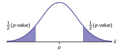
Figure 9.12

38 a right-tailed test

40 a left-tailed test

42 This is a left-tailed test.

44 This is a two-tailed test.

45

a. H0: μ = 34; Ha: μ ≠ 34

b. H0: p ≤ 0.60; Ha: p > 0.60

c. H0: μ ≥ 100,000; Ha: μ < 100,000 d. H0: p = 0.29; Ha: p ≠ 0.29

e. H0: p = 0.05; Ha: p < 0.05 f. H0: μ ≤ 10; Ha: μ > 10

g. H0: p = 0.50; Ha: p ≠ 0.50

h. H0: μ = 6; Ha: μ ≠ 6

i. H0: p ≥ 0.11; Ha: p < 0.11

j. H0: μ ≤ 20,000; Ha: μ > 20,000

47 c

49

• Type I error: We conclude that the mean is not 34 years, when it really is 34 years. Type II error: We conclude that the mean is 34 years, when in fact it really is not 34 years.
• Type I error: We conclude that more than 60% of Americans vote in presidential elections, when the actual percentage is at most 60%.Type II error: We conclude that at most 60% of Americans vote in presidential elections when, in fact, more than 60% do.
• Type I error: We conclude that the mean starting salary is less than $100,000, when it really is at least $100,000. Type II error: We conclude that the mean starting salary is at least $100,000 when, in fact, it is less than $100,000.
• Type I error: We conclude that the proportion of high school seniors who get drunk each month is not 29%, when it really is 29%. Type II error: We conclude that the proportion of high school seniors who get drunk each month is 29% when, in fact, it is not 29%.
• Type I error: We conclude that fewer than 5% of adults ride the bus to work in Los Angeles, when the percentage that do is really 5% or more. Type II error: We conclude that 5% or more adults ride the bus to work in Los Angeles when, in fact, fewer that 5% do.
• Type I error: We conclude that the mean number of cars a person owns in his or her lifetime is more than 10, when in reality it is not more than 10. Type II error: We conclude that the mean number of cars a person owns in his or her

lifetime is not more than 10 when, in fact, it is more than 10.

• Type I error: We conclude that the proportion of Americans who prefer to live away from cities is not about half, though the actual proportion is about half. Type II error: We conclude that the proportion of Americans who prefer to live away from cities is half when, in fact, it is not half.
• Type I error: We conclude that the duration of paid vacations each year for Europeans is not six weeks, when in fact it is six weeks. Type II error: We conclude that the duration of paid vacations each year for Europeans is six weeks when, in fact, it is not.
• Type I error: We conclude that the proportion is less than 11%, when it is really at least 11%. Type II error: We conclude that the proportion of women who develop breast cancer is at least 11%, when in fact it is less than 11%.
• Type I error: We conclude that the average tuition cost at private universities is more than $20,000, though in reality it is at most $20,000. Type II error: We conclude that the average tuition cost at private universities is at most $20,000 when, in fact, it is more than $20,000.

51 b

53 d

55 d

56

a. H0: μ ≥ 50,000 b. Ha: μ < 50,000

• Let X¯ = the average lifespan of a brand of tires.
• normal distribution e. z = -2.315
• p-value = 0.0103
• Check student’s solution.
• i. alpha: 0.05
• Decision: Reject the null hypothesis.
• Reason for decision: The p-value is less than 0.05.
• Conclusion: There is sufficient evidence to conclude that the mean lifespan of the tires is less than 50,000 miles. i. (43,537, 49,463)

58

a. H0: μ = $1.00

b. Ha: μ ≠ $1.00

• Let X¯ = the average cost of a daily newspaper.
• normal distribution e. z = –0.866
• p-value = 0.3865
• Check student’s solution.
• i. Alpha: 0.01
• Decision: Do not reject the null hypothesis.
• Reason for decision: The p-value is greater than 0.01.
• Conclusion: There is sufficient evidence to support the claim that the mean cost of daily papers is $1. The mean cost could be $1.

i. ($0.84, $1.06)

This OpenStax book is available for free at http://cnx.org/content/col11776/1.33

60

a. H0: μ = 10

b. Ha: μ ≠ 10

• Let X¯ the mean number of sick days an employee takes per year.
• Student’s t-distribution e. t = –1.12
• p-value = 0.300
• Check student’s solution.
• i. Alpha: 0.05
• Decision: Do not reject the null hypothesis.
• Reason for decision: The p-value is greater than 0.05.
• Conclusion: At the 5% significance level, there is insufficient evidence to conclude that the mean number of sick days is not ten.

i. (4.9443, 11.806)

62

a. H0: p ≥ 0.6

• Ha: p < 0.6
• Let P′ = the proportion of students who feel more enriched as a result of taking Elementary Statistics.
• normal for a single proportion e. 1.12
• p-value = 0.1308
• Check student’s solution.
• i. Alpha: 0.05
• Decision: Do not reject the null hypothesis.
• Reason for decision: The p-value is greater than 0.05.
• Conclusion: There is insufficient evidence to conclude that less than 60 percent of her students feel more enriched.
• Confidence Interval: (0.409, 0.654)

The “plus-4s” confidence interval is (0.411, 0.648)

64

a. H0: μ = 4

• Ha: μ ≠ 4
• Let X¯ the average I.Q. of a set of brown trout.
• two-tailed Student’s t-test e. t = 1.95
• p-value = 0.076
• Check student’s solution.
• i. Alpha: 0.05
• Decision: Reject the null hypothesis.
• Reason for decision: The p-value is greater than 0.05

• Conclusion: There is insufficient evidence to conclude that the average IQ of brown trout is not four. i. (3.8865,5.9468)

66

a. H0: p ≥ 0.13 b. Ha: p < 0.13

• Let P′ = the proportion of Americans who have seen or sensed angels
• normal for a single proportion e. –2.688
• p-value = 0.0036
• Check student’s solution.
• i. alpha: 0.05
• Decision: Reject the null hypothesis.
• Reason for decision: The p-value is less than 0.05.
• Conclusion: There is sufficient evidence to conclude that the percentage of Americans who have seen or sensed an angel is less than 13%.

i. (0, 0.0623).

The“plus-4s” confidence interval is (0.0022, 0.0978)

69

a. H0: p = 0.14 b. Ha: p < 0.14

• Let P′ = the proportion of NYC residents that smoke.
• normal for a single proportion e. –0.2756
• p-value = 0.3914
• Check student’s solution.
• i. alpha: 0.05
• Decision: Do not reject the null hypothesis.
• Reason for decision: The p-value is greater than 0.05.
• At the 5% significance level, there is insufficient evidence to conclude that the proportion of NYC residents who smoke is less than 0.14.
• Confidence Interval: (0.0502, 0.2070): The “plus-4s” confidence interval (see chapter 8) is (0.0676, 0.2297).

71

a. H0: μ = 69,110 b. Ha: μ > 69,110

• Let X¯ = the mean salary in dollars for California registered nurses.
• Student’s t-distribution e. t = 1.719
• p-value: 0.0466
• Check student’s solution.
• i. Alpha: 0.05
• Decision: Reject the null hypothesis.

This OpenStax book is available for free at http://cnx.org/content/col11776/1.33

• Reason for decision: The p-value is less than 0.05.
• Conclusion: At the 5% significance level, there is sufficient evidence to conclude that the mean salary of California registered nurses exceeds $69,110.

i. ($68,757, $73,485)

73 c

75 c

77

a. H0: p = 0.488 Ha: p ≠ 0.488

• p-value = 0.0114
• alpha = 0.05
• Reject the null hypothesis.
• At the 5% level of significance, there is enough evidence to conclude that 48.8% of families own stocks.
• The survey does not appear to be accurate.

79

a. H0: p = 0.517 Ha: p ≠ 0.517

b. p-value = 0.9203.

• alpha = 0.05.
• Do not reject the null hypothesis.
• At the 5% significance level, there is not enough evidence to conclude that the proportion of homes in Kentucky that are heated by natural gas is 0.517.
• However, we cannot generalize this result to the entire nation. First, the sample’s population is only the state of Kentucky. Second, it is reasonable to assume that homes in the extreme north and south will have extreme high usage and low usage, respectively. We would need to expand our sample base to include these possibilities if we wanted to generalize this claim to the entire nation.

81

a. H0: µ ≥ 11.52 Ha: µ < 11.52

• p-value = 0.000002 which is almost 0.
• alpha = 0.05.
• Reject the null hypothesis.
• At the 5% significance level, there is enough evidence to conclude that the mean amount of summer rain in the northeaster US is less than 11.52 inches, on average.
• We would make the same conclusion if alpha was 1% because the p-value is almost 0.

83

a. H0: µ ≤ 5.8 Ha: µ > 5.8

• p-value = 0.9987
• alpha = 0.05
• Do not reject the null hypothesis.
• At the 5% level of significance, there is not enough evidence to conclude that a woman visits her doctor, on average, more than 5.8 times a year.

85

a. H0: µ ≥ 150 Ha: µ < 150

• p-value = 0.0622

• alpha = 0.01
• Do not reject the null hypothesis.
• At the 1% significance level, there is not enough evidence to conclude that freshmen students study less than 2.5 hours per day, on average.
• The student academic group’s claim appears to be correct.

This OpenStax book is available for free at http://cnx.org/content/col11776/1.33