10 10 | HYPOTHESIS TESTING WITH TWO SAMPLES

Figure 10.1 If you want to test a claim that involves two groups (the types of breakfasts eaten east and west of the Mississippi River) you can use a slightly different technique when conducting a hypothesis test. (credit: Chloe Lim)

Introduction

Studies often compare two groups. For example, researchers are interested in the effect aspirin has in preventing heart attacks. Over the last few years, newspapers and magazines have reported various aspirin studies involving two groups. Typically, one group is given aspirin and the other group is given a placebo. Then, the heart attack rate is studied over several years.

There are other situations that deal with the comparison of two groups. For example, studies compare various diet and exercise programs. Politicians compare the proportion of individuals from different income brackets who might vote for them. Students are interested in whether SAT or GRE preparatory courses really help raise their scores. Many business applications require comparing two groups. It may be the investment returns of two different investment strategies, or the differences in production efficiency of different management styles.

To compare two means or two proportions, you work with two groups. The groups are classified either as independent or

matched pairs. Independent groups consist of two samples that are independent, that is, sample values selected from one

population are not related in any way to sample values selected from the other population. Matched pairs consist of two samples that are dependent. The parameter tested using matched pairs is the population mean. The parameters tested using independent groups are either population means or population proportions of each group.

| Comparing Two Independent Population Means

The comparison of two independent population means is very common and provides a way to test the hypothesis that the two groups differ from each other. Is the night shift less productive than the day shift, are the rates of return from fixed asset investments different from those from common stock investments, and so on? An observed difference between two sample means depends on both the means and the sample standard deviations. Very different means can occur by chance if there is great variation among the individual samples. The test statistic will have to account for this fact. The test comparing two independent population means with unknown and possibly unequal population standard deviations is called the Aspin- Welch t-test. The degrees of freedom formula we will see later was developed by Aspin-Welch.

When we developed the hypothesis test for the mean and proportions we began with the Central Limit Theorem. We recognized that a sample mean came from a distribution of sample means, and sample proportions came from the sampling distribution of sample proportions. This made our sample parameters, the sample means and sample proportions, into random variables. It was important for us to know the distribution that these random variables came from. The Central Limit Theorem gave us the answer: the normal distribution. Our Z and t statistics came from this theorem. This provided us with the solution to our question of how to measure the probability that a sample mean came from a distribution with a particular hypothesized value of the mean or proportion. In both cases that was the question: what is the probability that the mean (or proportion) from our sample data came from a population distribution with the hypothesized value we are interested in?

Now we are interested in whether or not two samples have the same mean. Our question has not changed: Do these two samples come from the same population distribution? To approach this problem we create a new random variable. We recognize that we have two sample means, one from each set of data, and thus we have two random variables coming from two unknown distributions. To solve the problem we create a new random variable, the difference between the sample means. This new random variable also has a distribution and, again, the Central Limit Theorem tells us that this new distribution is normally distributed, regardless of the underlying distributions of the original data. A graph may help to understand this concept.

This OpenStax book is available for free at http://cnx.org/content/col11776/1.33

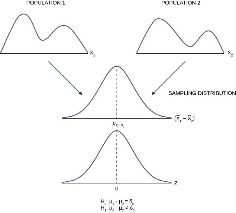
Figure 10.2

Pictured are two distributions of data, X1 and X2, with unknown means and standard deviations. The second panel shows the sampling distribution of the newly created random variable ( X– 1 – X– 2 ). This distribution is the theoretical distribution

of many many sample means from population 1 minus sample means from population 2. The Central Limit Theorem tells us that this theoretical sampling distribution of differences in sample means is normally distributed, regardless of the distribution of the actual population data shown in the top panel. Because the sampling distribution is normally distributed, we can develop a standardizing formula and calculate probabilities from the standard normal distribution in the bottom panel, the Z distribution. We have seen this same analysis before in Chapter 7 Figure 7.2 .

2⎠
The Central Limit Theorem, as before, provides us with the standard deviation of the sampling distribution, and further, that the expected value of the mean of the distribution of differences in sample means is equal to the differences in the population means. Mathematically this can be stated:

⎝
E⎛µ x–

1 – µ x–

⎞ = µ1 – µ2

Because we do not know the population standard deviations, we estimate them using the two sample standard deviations from our independent samples. For the hypothesis test, we calculate the estimated standard deviation, or standard error,

of the difference in sample means, X¯ 1 – X¯ 2 .

(s1 )2 + (s2 )2n1n2

The standard error is:

We remember that substituting the sample variance for the population variance when we did not have the population variance was the technique we used when building the confidence interval and the test statistic for the test of hypothesis for a single mean back in Confidence Intervals and Hypothesis Testing with One Sample. The test statistic (t-score)

is calculated as follows:

( x¯ 1 – x¯ 2 ) – δ0(s1 )2 + (s2 )2n1n2
tc =

where:

• s1 and s2, the sample standard deviations, are estimates of σ1 and σ2, respectively and
• σ1 and σ1 are the unknown population standard deviations.
• x¯ 1 and x¯ 2 are the sample means. μ1 and μ2 are the unknown population means.

The number of degrees of freedom (df) requires a somewhat complicated calculation. The df are not always a whole number. The test statistic above is approximated by the Student’s t-distribution with df as follows:

Degrees of freedom

⎛ (s1)2(s2)2⎞ 2

d f =

⎜ n1 +

2

⎟

⎝
n2 ⎠

2

⎛ 1 ⎞⎛ (s1)2⎞⎛ 1 ⎞⎛ (s2)2⎞

⎝n1 – 1⎠⎜

⎟

⎝
⎝
n1 ⎠

+ ⎝n2 – 1⎠⎜

⎟

n2 ⎠

When both sample sizes n1 and n2 are 30 or larger, the Student’s t approximation is very good. If each sample has more than 30 observations then the degrees of freedom can be calculated as n1 + n2 – 2.

The format of the sampling distribution, differences in sample means, specifies that the format of the null and alternative hypothesis is:

H0 : µ1 – µ2 = δ0

Ha : µ1 – µ2 ≠ δ0

where δ0 is the hypothesized difference between the two means. If the question is simply “is there any difference between the means?” then δ0 = 0 and the null and alternative hypotheses becomes:

H0 : µ1 = µ2

Ha : µ1 ≠ µ2

An example of when δ0 might not be zero is when the comparison of the two groups requires a specific difference for the decision to be meaningful. Imagine that you are making a capital investment. You are considering changing from your current model machine to another. You measure the productivity of your machines by the speed they produce the product. It may be that a contender to replace the old model is faster in terms of product throughput, but is also more expensive. The second machine may also have more maintenance costs, setup costs, etc. The null hypothesis would be set up so that the new machine would have to be better than the old one by enough to cover these extra costs in terms of speed and cost of production. This form of the null and alternative hypothesis shows how valuable this particular hypothesis test can be. For most of our work we will be testing simple hypotheses asking if there is any difference between the two distribution means.

Example 10.1 Independent groupsThe Kona Iki Corporation produces coconut milk. They take coconuts and extract the milk inside by drilling a hole and pouring the milk into a vat for processing. They have both a day shift (called the B shift) and a night shift (called the G shift) to do this part of the process. They would like to know if the day shift and the night shift are equally efficient in processing the coconuts. A study is done sampling 9 shifts of the G shift and 16 shifts of the B shift. The results of the number of hours required to process 100 pounds of coconuts is presented in Table10.1. A study is done and data are collected, resulting in the data in Table 10.1.

This OpenStax book is available for free at http://cnx.org/content/col11776/1.33

Table 10.1

Is there a difference in the mean amount of time for each shift to process 100 pounds of coconuts? Test at the 5% level of significance.

Solution 10.1

The population standard deviations are not known and cannot be assumed to equal each other. Let g be the subscript for the G Shift and b be the subscript for the B Shift. Then, μg is the population mean for G Shift and μb is the population mean for B Shift. This is a test of two independent groups, two population means.

Random variable: X¯ g − X¯ b = difference in the sample mean amount of time between the G Shift and the B Shift takes to process the coconuts.

H0: μg = μbH0: μg – μb = 0

Ha: μg ≠ μbHa: μg – μb ≠ 0

The words “the same” tell you H0 has an “=”. Since there are no other words to indicate Ha, is either faster or slower. This is a two tailed test.

Distribution for the test: Use tdf where df is calculated using the df formula for independent groups, two population means above. Using a calculator, df is approximately 18.8462.

Graph:

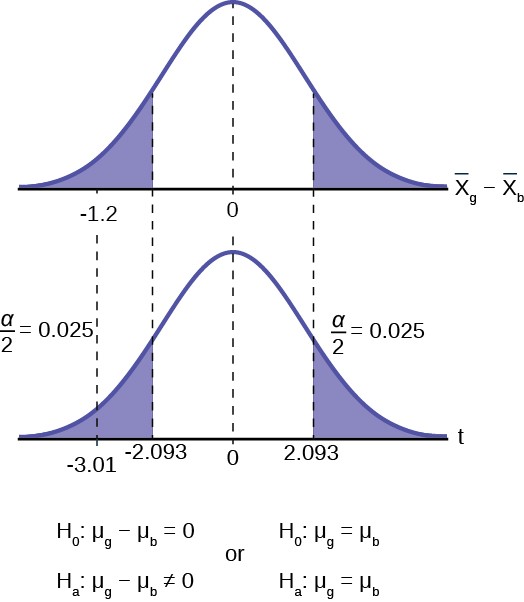
Figure 10.3

tc =

⎛X-⎝1 2⎠0− X- ⎞ − δS 2S 2n1 + n212
= -3.01

We next find the critical value on the t-table using the degrees of freedom from above. The critical value, 2.093, is found in the .025 column, this is α/2, at 19 degrees of freedom. (The convention is to round up the degrees of freedom to make the conclusion more conservative.) Next we calculate the test statistic and mark this on the t-distribution graph.

Make a decision: Since the calculated t-value is in the tail we cannot accept the null hypothesis that there is no difference between the two groups. The means are different.

The graph has included the sampling distribution of the differences in the sample means to show how the t- distribution aligns with the sampling distribution data. We see in the top panel that the calculated difference in the two means is -1.2 and the bottom panel shows that this is 3.01 standard deviations from the mean. Typically we do not need to show the sampling distribution graph and can rely on the graph of the test statistic, the t-distribution in this case, to reach our conclusion.

Conclusion: At the 5% level of significance, the sample data show there is sufficient evidence to conclude that the mean number of hours that the G Shift takes to process 100 pounds of coconuts is different from the B Shift (mean number of hours for the B Shift is greater than the mean number of hours for the G Shift).

This OpenStax book is available for free at http://cnx.org/content/col11776/1.33

NOTEWhen the sum of the sample sizes is larger than 30 (n1 + n2 > 30) you can use the normal distribution to approximate the Student’s t.

Example 10.2

A study is done to determine if Company A retains its workers longer than Company B. It is believed that Company A has a higher retention than Company B. The study finds that in a sample of 11 workers at Company A their average time with the company is four years with a standard deviation of 1.5 years. A sample of 9 workers at Company B finds that the average time with the company was 3.5 years with a standard deviation of 1 year. Test this proposition at the 1% level of significance.

a. Is this a test of two means or two proportions?

Solution 10.2

• two means because time is a continuous random variable.

• Are the populations standard deviations known or unknown?

Solution 10.2

• unknown

• Which distribution do you use to perform the test?

Solution 10.2

• Student’s t

• What is the random variable?

Solution 10.2

• X¯ A – X¯ B
• What are the null and alternate hypotheses?

Solution 10.2

e.

• Ho : µA ≤ µB
• Ha : µA > µB

• Is this test right-, left-, or two-tailed?

Solution 10.2

• right one-tailed test

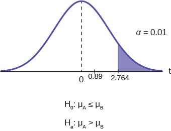
Figure 10.4

• What is the value of the test statistic?

⎛X-⎝1 2⎠0− X- ⎞ − δS 2S 2n1 + n212
Solution 10.2

tc =

= 0.89

• Can you accept/reject the null hypothesis?

Solution 10.2

• Cannot reject the null hypothesis that there is no difference between the two groups. Test statistic is not in the tail. The critical value of the t distribution is 2.764 with 10 degrees of freedom. This example shows how difficult it is to reject a null hypothesis with a very small sample. The critical values require very large test statistics to reach the tail.

Conclusion:

Solution 10.2

• At the 1% level of significance, from the sample data, there is not sufficient evidence to conclude that the retention of workers at Company A is longer than Company B, on average.

Example 10.3An interesting research question is the effect, if any, that different types of teaching formats have on the grade outcomes of students. To investigate this issue one sample of students’ grades was taken from a hybrid class and another sample taken from a standard lecture format class. Both classes were for the same subject. The mean course grade in percent for the 35 hybrid students is 74 with a standard deviation of 16. The mean grades of the 40 students form the standard lecture class was 76 percent with a standard deviation of 9. Test at 5% to see if there is any significant difference in the population mean grades between standard lecture course and hybrid class.

This OpenStax book is available for free at http://cnx.org/content/col11776/1.33

Solution 10.3

We begin by noting that we have two groups, students from a hybrid class and students from a standard lecture format class. We also note that the random variable, what we are interested in, is students’ grades, a continuous random variable. We could have asked the research question in a different way and had a binary random variable. For example, we could have studied the percentage of students with a failing grade, or with an A grade. Both of these would be binary and thus a test of proportions and not a test of means as is the case here. Finally, there is no presumption as to which format might lead to higher grades so the hypothesis is stated as a two-tailed test.

H0: µ1 = µ2

Ha: µ1 ≠ µ2

⎞
As would virtually always be the case, we do not know the population variances of the two distributions and thus our test statistic is:

⎛ x¯ 1 − x¯ 2 − δ0

(74 − 76) − 0

n1n2s2 + s2
tc = ⎝

⎠=

162 + 92

= −0.65

3540

To determine the critical value of the Student’s t we need the degrees of freedom. For this case we use: df = n1

+ n2 – 2 = 35 + 40 -2 = 73. This is large enough to consider it the normal distribution thus ta/2 = 1.96. Again as always we determine if the calculated value is in the tail determined by the critical value. In this case we do not even need to look up the critical value: the calculated value of the difference in these two average grades is not even one standard deviation apart. Certainly not in the tail.

Conclusion: Cannot reject the null at α=5%. Therefore, evidence does not exist to prove that the grades in hybrid and standard classes differ.

| Cohen’s Standards for Small, Medium, and Large Effect Sizes

Cohen’s d is a measure of “effect size” based on the differences between two means. Cohen’s d, named for United States statistician Jacob Cohen, measures the relative strength of the differences between the means of two populations based on sample data. The calculated value of effect size is then compared to Cohen’s standards of small, medium, and large effect sizes.

Table 10.2 Cohen’s Standard Effect Sizes

s pooled
Cohen’s d is the measure of the difference between two means divided by the pooled standard deviation: d = x¯ 1 – x¯ 2

(n1 – 1)s2 + (n2 – 1)s2n1 + n2 – 212
where s pooled =

It is important to note that Cohen’s d does not provide a level of confidence as to the magnitude of the size of the effect comparable to the other tests of hypothesis we have studied. The sizes of the effects are simply indicative.

Example 10.4Calculate Cohen’s d for ???. Is the size of the effect small, medium, or large? Explain what the size of the effect means for this problem.Solution 10.4x̅1 = 4 s1 = 1.5 n1 = 11x̅2 = 3.5 s2 = 1 n2 = 9d = 0.384The effect is small because 0.384 is between Cohen’s value of 0.2 for small effect size and 0.5 for medium effect size. The size of the differences of the means for the two companies is small indicating that there is not a significant difference between them.

| Test for Differences in Means: Assuming Equal Population Variances

⎞
Typically we can never expect to know any of the population parameters, mean, proportion, or standard deviation. When testing hypotheses concerning differences in means we are faced with the difficulty of two unknown variances that play a critical role in the test statistic. We have been substituting the sample variances just as we did when testing hypotheses for a single mean. And as we did before, we used a Student’s t to compensate for this lack of information on the population variance. There may be situations, however, when we do not know the population variances, but we can assume that the two populations have the same variance. If this is true then the pooled sample variance will be smaller than the individual sample variances. This will give more precise estimates and reduce the probability of discarding a good null. The null and alternative hypotheses remain the same, but the test statistic changes to:

⎛ x¯ 1 − x¯ 2 − δ0

Sp+2 ⎛⎝nn1112⎠⎞
tc = ⎝⎠

where Sp2 is the pooled variance given by the formula:

⎛n

− 1⎞s1 + ⎛n − 1⎞s2

Sp2 = ⎝ 1

⎠ 2⎝ 2⎠ 2

n + n − 2

12

Example 10.5A drug trial is attempted using a real drug and a pill made of just sugar. 18 people are given the real drug in hopes of increasing the production of endorphins. The increase in endorphins is found to be on average 8 micrograms per person, and the sample standard deviation is 5.4 micrograms. 11 people are given the sugar pill, and their average endorphin increase is 4 micrograms with a standard deviation of 2.4. From previous research on endorphins it is determined that it can be assumed that the variances within the two samples can be assumed to be the same. Test at 5% to see if the population mean for the real drug had a significantly greater impact on the endorphins than the population mean with the sugar pill.Solution 10.5First we begin by designating one of the two groups Group 1 and the other Group 2. This will be needed to keep track of the null and alternative hypotheses. Let’s set Group 1 as those who received the actual new medicine being tested and therefore Group 2 is those who received the sugar pill. We can now set up the null and alternative hypothesis as:

This OpenStax book is available for free at http://cnx.org/content/col11776/1.33

H0: µ1 ≤ µ2 H1: µ1 > µ2

This is set up as a one-tailed test with the claim in the alternative hypothesis that the medicine will produce more endorphins than the sugar pill. We now calculate the test statistic which requires us to calculate the pooled variance, Sp2 using the formula above.

tc =

= (8 − 4) − 0

⎛ x¯ 1 − x¯ 2⎠ − δ0⎝⎞Sp2 ⎛ 11 ⎞⎝n1 + n2⎠

⎛ = 2.3120.4933+
⎝ 11

1811

tα, allows us to compare the test statistic and the critical value.

tα = 1.703 at d f = n1 + n2 − 2 = 18 + 11 − 2 = 27

The test statistic is clearly in the tail, 2.31 is larger than the critical value of 1.703, and therefore we cannot maintain the null hypothesis. Thus, we conclude that there is significant evidence at the 95% level of confidence that the new medicine produces the effect desired.

| Comparing Two Independent Population Proportions

When conducting a hypothesis test that compares two independent population proportions, the following characteristics should be present:

• The two independent samples are random samples that are independent.
• The number of successes is at least five, and the number of failures is at least five, for each of the samples.
• Growing literature states that the population must be at least ten or even perhaps 20 times the size of the sample. This keeps each population from being over-sampled and causing biased results.

Comparing two proportions, like comparing two means, is common. If two estimated proportions are different, it may be due to a difference in the populations or it may be due to chance in the sampling. A hypothesis test can help determine if a difference in the estimated proportions reflects a difference in the two population proportions.

Like the case of differences in sample means, we construct a sampling distribution for differences in sample proportions:

⎛p‘ – p‘ ⎞ where p‘ = X A and p‘ = X B are the sample proportions for the two sets of data in question. XA and XB

⎝ AB⎠

• 
  n A
• 
  n B

are the number of successes in each sample group respectively, and nA and nB are the respective sample sizes from the two groups. Again we go the Central Limit theorem to find the distribution of this sampling distribution for the differences in sample proportions. And again we find that this sampling distribution, like the ones past, are normally distributed as proved by the Central Limit Theorem, as seen in Figure 10.5 .

Figure 10.5

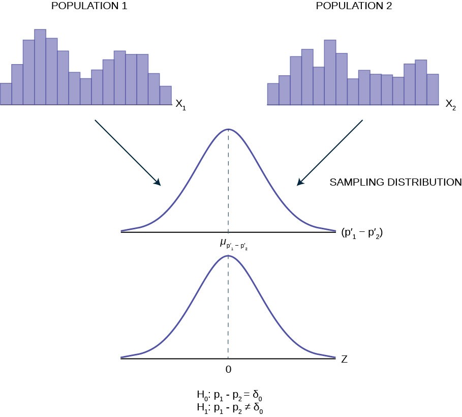
Generally, the null hypothesis allows for the test of a difference of a particular value, 𝛿0, just as we did for the case of differences in means.

H0 : p1 − p2 = 𝛿 0

H1 : p1 − p2 ≠ 𝛿 0

Most common, however, is the test that the two proportions are the same. That is,

H0 : pA = pB

Ha : pA ≠ pB

To conduct the test, we use a pooled proportion, pc.

The pooled proportion is calculated as follows:

pc =
x A + xB n A + nB

This OpenStax book is available for free at http://cnx.org/content/col11776/1.33

(p′A − p′B) − δ0pc(1 − pc)(n1 + n1 )AB
The test statistic (z-score) is:

Zc =

where δ0 is the hypothesized differences between the two proportions and pc is the pooled variance from the formula above.

Example 10.6

A bank has recently acquired a new branch and thus has customers in this new territory. They are interested in the default rate in their new territory. They wish to test the hypothesis that the default rate is different from their current customer base. They sample 200 files in area A, their current customers, and find that 20 have defaulted. In area B, the new customers, another sample of 200 files shows 12 have defaulted on their loans. At a 10% level of significance can we say that the default rates are the same or different?

Solution 10.6

This is a test of proportions. We know this because the underlying random variable is binary, default or not default. Further, we know it is a test of differences in proportions because we have two sample groups, the current customer base and the newly acquired customer base. Let A and B be the subscripts for the two customer groups. Then pA and pB are the two population proportions we wish to test.

Random Variable:

P′A – P′B = difference in the proportions of customers who defaulted in the two groups.

H0 : p A = pB

Ha : p A ≠ pB

The words “is a difference” tell you the test is two-tailed.

Distribution for the test: Since this is a test of two binomial population proportions, the distribution is normal:

pc = x A + xB = 20 + 12 = 0.08 1 – pc = 0.92

n A + nB

200 + 200

(p′A – p′B) = 0.04 follows an approximate normal distribution.

Estimated proportion for group A: p′ A = x A = 20

= 0.1

n A200

Estimated proportion for group B: p′B = xB = 12

= 0.06

nB200

The estimated difference between the two groups is : p′A – p′B = 0.1 – 0.06 = 0.04.

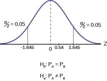
Figure 10.6

⎛P′

A
− P′ ⎞ − δ

B
Zc =⎝ A

⎛B⎠

0 ⎞ = 0.54

Pc(1 − Pc)⎝n1

+ n1 ⎠

The calculated test statistic is .54 and is not in the tail of the distribution.

Make a decision: Since the calculate test statistic is not in the tail of the distribution we cannot reject H0.

Conclusion: At a 1% level of significance, from the sample data, there is not sufficient evidence to conclude that there is a difference between the proportions of customers who defaulted in the two groups.

10.6 Two types of valves are being tested to determine if there is a difference in pressure tolerances. Fifteen out of a random sample of 100 of Valve A cracked under 4,500 psi. Six out of a random sample of 100 of Valve B cracked under 4,500 psi. Test at a 5% level of significance.

| Two Population Means with Known Standard Deviations

Even though this situation is not likely (knowing the population standard deviations is very unlikely), the following example illustrates hypothesis testing for independent means with known population standard deviations. The sampling distribution

fo–r the–difference between the means is normal in accordance with the central limit theorem. The random variable is

X1 – X2 . The normal distribution has the following format:

(σ1)2 + (σ2)2n1n2

The standard deviation is:

This OpenStax book is available for free at http://cnx.org/content/col11776/1.33

( x 1 – x 2) – δ0(σ1)2 + (σ2)2n1n2
The test sta–tistic–(z-score) is:

Zc =

Example 10.7

Independent groups, population standard deviations known: The mean lasting time of two competing floor waxes is to be compared. Twenty floors are randomly assigned to test each wax. Both populations have a normal distributions. The data are recorded in Table 10.3.

Table 10.3

Does the data indicate that wax 1 is more effective than wax 2? Test at a 5% level of significance.

Solution 10.7

This is a test of two independent groups, two population means, population standard deviations known.

Random Variable: X– 1 – X– 2 = difference in the mean number of months the competing floor waxes last.

H0 : µ 1 ≤ µ 2

Ha : µ 1 > µ 2

The words “is more effective” says that wax 1 lasts longer than wax 2, on average. “Longer” is a “>” symbol and goes into Ha. Therefore, this is a right-tailed test.

Distribution for the test: The population standard deviations are known so the distribution is normal. Using the formula for the test statistic we find the calculated value for the problem.

== 0.1
Z⎛µ 1 – µ ⎞ – δ0

⎝2⎠

cσ 2σ 2

n1 + n2

12

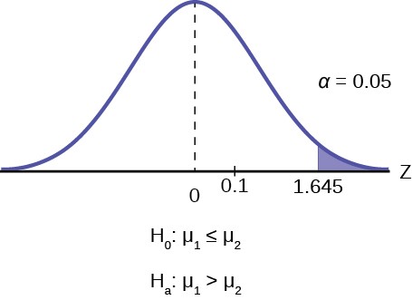
Figure 10.7

The estimated difference between he two means is : X– 1 – X– 2 = 3 – 2.9 = 0.1

Compare calculated value and critical value and Zα: We mark the calculated value on the graph and find the the calculate value is not in the tail therefore we cannot reject the null hypothesis.

Make a decision: the calculated value of the test statistic is not in the tail, therefore you cannot reject H0.

10.7 The means of the number of revolutions per minute of two competing engines are to be compared. Thirty engines are randomly assigned to be tested. Both populations have normal distributions. Table 10.4 shows the result. Do the data indicate that Engine 2 has higher RPM than Engine 1? Test at a 5% level of significance.Table 10.4
Conclusion: At the 5% level of significance, from the sample data, there is not sufficient evidence to conclude that the mean time wax 1 lasts is longer (wax 1 is more effective) than the mean time wax 2 lasts.

Example 10.8An interested citizen wanted to know if Democratic U. S. senators are older than Republican U.S. senators, on average. On May 26 2013, the mean age of 30 randomly selected Republican Senators was 61 years 247 days old (61.675 years) with a standard deviation of 10.17 years. The mean age of 30 randomly selected Democratic senators was 61 years 257 days old (61.704 years) with a standard deviation of 9.55 years.

This OpenStax book is available for free at http://cnx.org/content/col11776/1.33

Do the data indicate that Democratic senators are older than Republican senators, on average? Test at a 5% level of significance.

Solution 10.8

This is a test of two independent groups, two population means. The population standard deviations are unknown, but the sum of the sample sizes is 30 + 30 = 60, which is greater than 30, so we can use the normal approximation to the Student’s-t distribution. Subscripts: 1: Democratic senators 2: Republican senators

Random variable: X– 1 – X– 2 = difference in the mean age of Democratic and Republican U.S. senators.

H0 : µ 1 ≤ µ 2 H0 : µ 1 – µ 2 ≤ 0

Ha : µ 1 > µ 2 Ha : µ 1 – µ 2 > 0

The words “older than” translates as a “>” symbol and goes into Ha. Therefore, this is a right-tailed test.

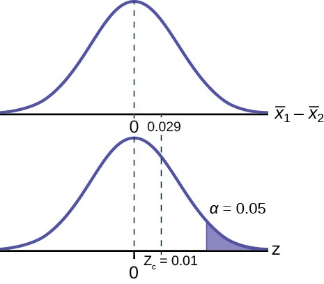
Figure 10.8

Make a decision: The p-value is larger than 5%, therefore we cannot reject the null hypothesis. By calculating the test statistic we would find that the test statistic does not fall in the tail, therefore we cannot reject the null hypothesis. We reach the same conclusion using either method of a making this statistical decision.

Conclusion: At the 5% level of significance, from the sample data, there is not sufficient evidence to conclude that the mean age of Democratic senators is greater than the mean age of the Republican senators.

| Matched or Paired Samples

In most cases of economic or business data we have little or no control over the process of how the data are gathered. In this sense the data are not the result of a planned controlled experiment. In some cases, however, we can develop data that are part of a controlled experiment. This situation occurs frequently in quality control situations. Imagine that the production rates of two machines built to the same design, but at different manufacturing plants, are being tested for differences in some production metric such as speed of output or meeting some production specification such as strength of the product. The test is the same in format to what we have been testing, but here we can have matched pairs for which we can test if

differences exist. Each observation has its matched pair against which differences are calculated. First, the differences in the metric to be tested between the two lists of observations must be calculated, and this is typically labeled with the letter “d.” Then, the average of these matched differences, X¯ d is calculated as is its standard deviation, Sd. We expect that the

standard deviation of the differences of the matched pairs will be smaller than unmatched pairs because presumably fewer differences should exist because of the correlation between the two groups.

When using a hypothesis test for matched or paired samples, the following characteristics may be present:

• Simple random sampling is used.
• Sample sizes are often small.
• Two measurements (samples) are drawn from the same pair of individuals or objects.
• Differences are calculated from the matched or paired samples.
• The differences form the sample that is used for the hypothesis test.
• Either the matched pairs have differences that come from a population that is normal or the number of differences is sufficiently large so that distribution of the sample mean of differences is approximately normal.

In a hypothesis test for matched or paired samples, subjects are matched in pairs and differences are calculated. The differences are the data. The population mean for the differences, μd, is then tested using a Student’s-t test for a single population mean with n – 1 degrees of freedom, where n is the number of differences, that is, the number of pairs not the number of observations.

The null and alternative hypotheses for this test are:

H0 : µd = 0

Ha : µd ≠ 0

–
The test statistic is:

s⎝ d ⎞
tc = x ⎛d − µd

n⎠

Example 10.9A company has developed a training program for its entering employees because they have become concerned with the results of the six-month employee review. They hope that the training program can result in better six- month reviews. Each trainee constitutes a “pair”, the entering score the employee received when first entering the firm and the score given at the six-month review. The difference in the two scores were calculated for each employee and the means for before and after the training program was calculated. The sample mean before the training program was 20.4 and the sample mean after the training program was 23.9. The standard deviation of the differences in the two scores across the 20 employees was 3.8 points. Test at the 10% significance level the null hypothesis that the two population means are equal against the alternative that the training program helps improve the employees’ scores.Solution 10.9The first step is to identify this as a two sample case: before the training and after the training. This differentiates this problem from simple one sample issues. Second, we determine that the two samples are “paired.” Each observation in the first sample has a paired observation in the second sample. This information tells us that the null and alternative hypotheses should be:H0 : µd ≤ 0Ha : µd > 0This form reflects the implied claim that the training course improves scores; the test is one-tailed and the claim is in the alternative hypothesis. Because the experiment was conducted as a matched paired sample rather than simply taking scores from people who took the training course those who didn’t, we use the matched pair test statistic:

This OpenStax book is available for free at http://cnx.org/content/col11776/1.33

Test Statistic: tc =

X¯ d − µd

Sd n

= (23.9 −⎛ 20⎞.4) − 0

3.8⎝⎠
20

= 4.12

In order to solve this equation, the individual scores, pre-training course and post-training course need to be used to calculate the individual differences. These scores are then averaged and the average difference is calculated:

X¯ d = x¯ 1 − x¯ 2

From these differences we can calculate the standard deviation across the individual differences:

Σ⎛d − X¯ ⎞2

n − 1
d
i
S = ⎝ id ⎠ where d

= x1i

• 
  x2i

Example 10.10A study was conducted to investigate the effectiveness of hypnotism in reducing pain. Results for randomly selected subjects are shown in Table 10.4. A lower score indicates less pain. The “before” value is matched to an “after” value and the differences are calculated. Are the sensory measurements, on average, lower after hypnotism? Test at a 5% significance level.Table 10.5Solution 10.10Corresponding “before” and “after” values form matched pairs. (Calculate “after” – “before.”)Table 10.6
We can now compare the calculated value of the test statistic, 4.12, with the critical value. The critical value is a Student’s t with degrees of freedom equal to the number of pairs, not observations, minus 1. In this case 20 pairs and at 90% confidence level ta/2 = ±1.729 at df = 20 – 1 = 19. The calculated test statistic is most certainly in the tail of the distribution and thus we cannot accept the null hypothesis that there is no difference from the training program. Evidence seems indicate that the training aids employees in gaining higher scores.

The data for the test are the differences: {0.2, –4.1, –1.6, –1.8, –3.2, –2, –2.9, –9.6}

The sample mean and sample standard deviation of the differences are: x– d = –3.13 and sd = 2.91 Verify these values.

Let µd be the population mean for the differences. We use the subscript d to denote “differences.”

Random variable: X– d = the mean difference of the sensory measurements

H0: μd ≥ 0

The null hypothesis is zero or positive, meaning that there is the same or more pain felt after hypnotism. That means the subject shows no improvement. μd is the population mean of the differences.)

Ha: μd < 0

The alternative hypothesis is negative, meaning there is less pain felt after hypnotism. That means the subject shows improvement. The score should be lower after hypnotism, so the difference ought to be negative to indicate improvement.

Distribution for the test: The distribution is a Student’s t with df = n – 1 = 8 – 1 = 7. Use t7. (Notice that the test is for a single population mean.)

Calculate the test statistic and look up the critical value using the Student’s-t distribution: The calculated value of the test statistic is 3.06 and the critical value of the t distribution with 7 degrees of freedom at the 5% level of confidence is 1.895 with a one-tailed test.

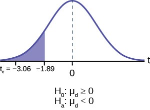
Figure 10.9

X– d is the random variable for the differences.

The sample mean and sample standard deviation of the differences are:

–x d = –3.13

–s d = 2.91

Compare the critical value for alpha against the calculated test statistic.

The conclusion from using the comparison of the calculated test statistic and the critical value will gives us the result. In this question the calculated test statistic is 3.06 and the critical value is 1.895. The test statistic is clearly in the tail and thus we cannot accept the null hypotheses that there is no difference between the two situations, hypnotized and not hypnotized.

Make a decision: Cannot accept the null hypothesis, H0. This means that μd < 0 and there is a statistically significant improvement.

This OpenStax book is available for free at http://cnx.org/content/col11776/1.33

Conclusion: At a 5% level of significance, from the sample data, there is sufficient evidence to conclude that the sensory measurements, on average, are lower after hypnotism. Hypnotism appears to be effective in reducing pain.

Example 10.11

A college football coach was interested in whether the college’s strength development class increased his players’ maximum lift (in pounds) on the bench press exercise. He asked four of his players to participate in a study. The amount of weight they could each lift was recorded before they took the strength development class. After completing the class, the amount of weight they could each lift was again measured. The data are as follows:

Table 10.7

The coach wants to know if the strength development class makes his players stronger, on average.

Record the differences data. Calculate the differences by subtracting the amount of weight lifted prior to the class from the weight lifted after completing the class. The data for the differences are: {90, 11, -8, -8}.

–x d = 21.3, sd = 46.7

Using the difference data, this becomes a test of a single mean.

Define the random variable: X– d mean difference in the maximum lift per player. The distribution for the hypothesis test is a student’s t with 3 degrees of freedom.

H0: μd ≤ 0, Ha: μd > 0

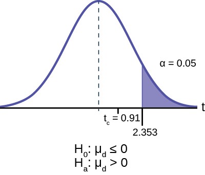
Figure 10.10

Calculate the test statistic look up the critical value: Critical value of the test statistic is 0.91. The critical value of the student’s t at 5% level of significance and 3 degrees of freedom is 2.353.

Decision: If the level of significance is 5%, we cannot reject the null hypothesis, because the calculated value of the test statistic is not in the tail.

What is the conclusion?

At a 5% level of significance, from the sample data, there is not sufficient evidence to conclude that the strength development class helped to make the players stronger, on average.

This OpenStax book is available for free at http://cnx.org/content/col11776/1.33

KEY TERMS

Cohen’s d a measure of effect size based on the differences between two means. If d is between 0 and 0.2 then the effect is small. If d approaches is 0.5, then the effect is medium, and if d approaches 0.8, then it is a large effect.

Independent Groups two samples that are selected from two populations, and the values from one population are not related in any way to the values from the other population.

Matched Pairs two samples that are dependent. Differences between a before and after scenario are tested by testing one population mean of differences.

Pooled Variance a weighted average of two variances that can then be used when calculating standard error.

CHAPTER REVIEW

Comparing Two Independent Population Means

Two population means from independent samples where the population standard deviations are not known

• Random Variable: X– 1 − X– 2 = the difference of the sampling means
• Distribution: Student’s t-distribution with degrees of freedom (variances not pooled)

Cohen’s Standards for Small, Medium, and Large Effect Sizes

Cohen’s d is a measure of “effect size” based on the differences between two means.

It is important to note that Cohen’s d does not provide a level of confidence as to the magnitude of the size of the effect comparable to the other tests of hypothesis we have studied. The sizes of the effects are simply indicative.

Test for Differences in Means: Assuming Equal Population Variances

In situations when we do not know the population variances but assume the variances are the same, the pooled sample variance will be smaller than the individual sample variances.

This will give more precise estimates and reduce the probability of discarding a good null.

Comparing Two Independent Population Proportions

Test of two population proportions from independent samples.

• Random variable: p’ A – p’B = difference between the two estimated proportions
• Distribution: normal distribution

Two Population Means with Known Standard Deviations

A hypothesis test of two population means from independent samples where the population standard deviations are known (typically approximated with the sample standard deviations), will have these characteristics:

• Random variable: X– 1 − X– 2 = the difference of the means
• Distribution: normal distribution

Matched or Paired Samples

A hypothesis test for matched or paired samples (t-test) has these characteristics:

• Test the differences by subtracting one measurement from the other measurement

• Random Variable:

–x d = mean of the differences

• Distribution: Student’s-t distribution with n – 1 degrees of freedom
• If the number of differences is small (less than 30), the differences must follow a normal distribution.

• Two samples are drawn from the same set of objects.
• Samples are dependent.

FORMULA REVIEW

⎛n − 1⎞s1 + ⎛n

− 1⎞s2

10.1 Comparing Two Independent Population

Sp2 = ⎝ 1

⎠ 2⎝ 2⎠ 2

n + n − 2

Means12

(s1)2 + (s2)2n1n2
Standard error: SE =

(s1)2 + (s2)2n1n2
Test statistic (t-score): tc =

( x¯ 1 − x¯ 2) − δ0

10.4 Comparing Two Independent Population Proportions

n+ n
Pooled Proportion: pc = x A + xB

AB

(p′ − p′ )

Test Statistic (z-score): Zc =

AB

A
B
⎛⎞

Degrees of freedom:

⎝
⎛ (s1)2

(s2)2⎞ 2

where

pc(1 − pc)⎝n1

+ n1 ⎠

d f =

⎜ n1 +

2

⎟

n2 ⎠

2

p‘ and p‘ are the sample proportions, p A and pB are

⎛ 1 ⎞⎛ (s1)2⎞⎛ 1 ⎞⎛ (s2)2⎞AB

where:

⎝n1 − 1⎠⎜

⎟

⎝
⎝
n1 ⎠

+ ⎝n2 − 1⎠⎜

⎟

n2 ⎠

the population proportions,

Pc is the pooled proportion, and nA and nB are the sample sizes.

s1 and s2 are the sample standard deviations, and n1 and

n2 are the sample sizes.

x¯ 1 and x¯ 2 are the sample means.

10.2 Cohen’s Standards for Small, Medium, and Large Effect Sizes

Cohen’s d is the measure of effect size:

d =12
x¯ − x¯

(n1 − 1)s2 + (n2 − 1)s2n1 + n2 − 212
s pooled

TwoPopulationMeanswithKnown Standard Deviations

( –x 1 − –x 2) − δ0(σ1)2 + (σ2)2n1n2
Test Statistic (z-score):

Zc =

where:

σ1 and σ2 are the known population standard deviations.

n1 and n2 are the sample sizes. –x 1 and –x 2 are the

where s pooled =

sample means. μ1 and μ2 are the population means.

Matched or Paired Samples

10.3 Test for Differences in Means: Assuming Equal Population Variances

Test Statistic (t-score): tc =

–x d − µd

⎛sd ⎞

⎛ x¯ − x¯ ⎞ − δ

⎝ n⎠

Sp+2⎛⎝nn1112⎠⎞
tc = ⎝

12⎠0

where:

–x d is the mean of the sample differences. μd is the mean

where Sp2 is the pooled variance given by the formula:

PRACTICE

of the population differences. sd is the sample standard deviation of the differences. n is the sample size.

This OpenStax book is available for free at http://cnx.org/content/col11776/1.33

Comparing Two Independent Population Means

Use the following information to answer the next 15 exercises: Indicate if the hypothesis test is for

• independent group means, population standard deviations, and/or variances known
• independent group means, population standard deviations, and/or variances unknown
• matched or paired samples
• single mean
• two proportions
• single proportion
• It is believed that 70% of males pass their drivers test in the first attempt, while 65% of females pass the test in the first attempt. Of interest is whether the proportions are in fact equal.
• A new laundry detergent is tested on consumers. Of interest is the proportion of consumers who prefer the new brand over the leading competitor. A study is done to test this.
• A new windshield treatment claims to repel water more effectively. Ten windshields are tested by simulating rain without the new treatment. The same windshields are then treated, and the experiment is run again. A hypothesis test is conducted.
• The known standard deviation in salary for all mid-level professionals in the financial industry is $11,000. Company A and Company B are in the financial industry. Suppose samples are taken of mid-level professionals from Company A and from Company B. The sample mean salary for mid-level professionals in Company A is $80,000. The sample mean salary for mid-level professionals in Company B is $96,000. Company A and Company B management want to know if their mid- level professionals are paid differently, on average.
• The average worker in Germany gets eight weeks of paid vacation.
• According to a television commercial, 80% of dentists agree that Ultrafresh toothpaste is the best on the market.
• It is believed that the average grade on an English essay in a particular school system for females is higher than for males. A random sample of 31 females had a mean score of 82 with a standard deviation of three, and a random sample of 25 males had a mean score of 76 with a standard deviation of four.
• The league mean batting average is 0.280 with a known standard deviation of 0.06. The Rattlers and the Vikings belong to the league. The mean batting average for a sample of eight Rattlers is 0.210, and the mean batting average for a sample of eight Vikings is 0.260. There are 24 players on the Rattlers and 19 players on the Vikings. Are the batting averages of the Rattlers and Vikings statistically different?
• In a random sample of 100 forests in the United States, 56 were coniferous or contained conifers. In a random sample of 80 forests in Mexico, 40 were coniferous or contained conifers. Is the proportion of conifers in the United States statistically more than the proportion of conifers in Mexico?
• A new medicine is said to help improve sleep. Eight subjects are picked at random and given the medicine. The means hours slept for each person were recorded before starting the medication and after.
• It is thought that teenagers sleep more than adults on average. A study is done to verify this. A sample of 16 teenagers has a mean of 8.9 hours slept and a standard deviation of 1.2. A sample of 12 adults has a mean of 6.9 hours slept and a standard deviation of 0.6.
• Varsity athletes practice five times a week, on average.
• A sample of 12 in-state graduate school programs at school A has a mean tuition of $64,000 with a standard deviation of

$8,000. At school B, a sample of 16 in-state graduate programs has a mean of $80,000 with a standard deviation of $6,000. On average, are the mean tuitions different?

• A new WiFi range booster is being offered to consumers. A researcher tests the native range of 12 different routers under the same conditions. The ranges are recorded. Then the researcher uses the new WiFi range booster and records the new ranges. Does the new WiFi range booster do a better job?
• A high school principal claims that 30% of student athletes drive themselves to school, while 4% of non-athletes drive themselves to school. In a sample of 20 student athletes, 45% drive themselves to school. In a sample of 35 non-athlete students, 6% drive themselves to school. Is the percent of student athletes who drive themselves to school more than the percent of nonathletes?

Use the following information to answer the next three exercises: A study is done to determine which of two soft drinks has more sugar. There are 13 cans of Beverage A in a sample and six cans of Beverage B. The mean amount of sugar in Beverage A is 36 grams with a standard deviation of 0.6 grams. The mean amount of sugar in Beverage B is 38 grams with a standard deviation of 0.8 grams. The researchers believe that Beverage B has more sugar than Beverage A, on average. Both populations have normal distributions.

• Are standard deviations known or unknown?
• What is the random variable?
• Is this a one-tailed or two-tailed test?

Use the following information to answer the next 12 exercises: The U.S. Center for Disease Control reports that the mean life expectancy was 47.6 years for whites born in 1900 and 33.0 years for nonwhites. Suppose that you randomly survey death records for people born in 1900 in a certain county. Of the 124 whites, the mean life span was 45.3 years with a standard deviation of 12.7 years. Of the 82 nonwhites, the mean life span was 34.1 years with a standard deviation of 15.6 years. Conduct a hypothesis test to see if the mean life spans in the county were the same for whites and nonwhites.

• Is this a test of means or proportions?
• State the null and alternative hypotheses.
• H0:
• Ha:
• Is this a right-tailed, left-tailed, or two-tailed test?
• In symbols, what is the random variable of interest for this test?
• In words, define the random variable of interest for this test.
• Which distribution (normal or Student’s t) would you use for this hypothesis test?
• Explain why you chose the distribution you did for Exercise 10.24.
• Calculate the test statistic.
• Sketch a graph of the situation. Label the horizontal axis. Mark the hypothesized difference and the sample difference. Shade the area corresponding to the p-value.
• At a pre-conceived α = 0.05, what is your:
• Decision:
• Reason for the decision:
• Conclusion (write out in a complete sentence):
• Does it appear that the means are the same? Why or why not?

Comparing Two Independent Population Proportions

Use the following information for the next five exercises. Two types of phone operating system are being tested to determine if there is a difference in the proportions of system failures (crashes). Fifteen out of a random sample of 150 phones with OS1 had system failures within the first eight hours of operation. Nine out of another random sample of 150 phones with OS2 had system failures within the first eight hours of operation. OS2 is believed to be more stable (have fewer crashes) than OS1.

• Is this a test of means or proportions?
• What is the random variable?
• State the null and alternative hypotheses.
• What can you conclude about the two operating systems?

Use the following information to answer the next twelve exercises. In the recent Census, three percent of the U.S. population reported being of two or more races. However, the percent varies tremendously from state to state. Suppose that two random surveys are conducted. In the first random survey, out of 1,000 North Dakotans, only nine people reported being of two or more races. In the second random survey, out of 500 Nevadans, 17 people reported being of two or more races. Conduct a hypothesis test to determine if the population percents are the same for the two states or if the percent for Nevada is statistically higher than for North Dakota.

This OpenStax book is available for free at http://cnx.org/content/col11776/1.33

• Is this a test of means or proportions?
• State the null and alternative hypotheses.
• H0:
• Ha:
• Is this a right-tailed, left-tailed, or two-tailed test? How do you know?
• What is the random variable of interest for this test?
• In words, define the random variable for this test.
• Which distribution (normal or Student’s t) would you use for this hypothesis test?
• Explain why you chose the distribution you did for the Exercise 10.56.
• Calculate the test statistic.
• At a pre-conceived α = 0.05, what is your:
• Decision:
• Reason for the decision:
• Conclusion (write out in a complete sentence):
• Does it appear that the proportion of Nevadans who are two or more races is higher than the proportion of North Dakotans? Why or why not?

Two Population Means with Known Standard Deviations

Use the following information to answer the next five exercises. The mean speeds of fastball pitches from two different baseball pitchers are to be compared. A sample of 14 fastball pitches is measured from each pitcher. The populations have normal distributions. Table 10.8 shows the result. Scouters believe that Rodriguez pitches a speedier fastball.

Table 10.8

• What is the random variable?
• State the null and alternative hypotheses.
• What is the test statistic?
• At the 1% significance level, what is your conclusion?

Use the following information to answer the next five exercises. A researcher is testing the effects of plant food on plant growth. Nine plants have been given the plant food. Another nine plants have not been given the plant food. The heights of the plants are recorded after eight weeks. The populations have normal distributions. The following table is the result. The researcher thinks the food makes the plants grow taller.

Table 10.9

• Is the population standard deviation known or unknown?
• State the null and alternative hypotheses.
• At the 1% significance level, what is your conclusion?

Use the following information to answer the next five exercises. Two metal alloys are being considered as material for ball bearings. The mean melting point of the two alloys is to be compared. 15 pieces of each metal are being tested. Both populations have normal distributions. The following table is the result. It is believed that Alloy Zeta has a different melting point.

Table 10.10

• State the null and alternative hypotheses.
• Is this a right-, left-, or two-tailed test?
• At the 1% significance level, what is your conclusion?

Matched or Paired Samples

Use the following information to answer the next five exercises. A study was conducted to test the effectiveness of a software patch in reducing system failures over a six-month period. Results for randomly selected installations are shown in Table

10.11. The “before” value is matched to an “after” value, and the differences are calculated. The differences have a normal distribution. Test at the 1% significance level.

Table 10.11

• What is the random variable?
• State the null and alternative hypotheses.
• What conclusion can you draw about the software patch?

Use the following information to answer next five exercises. A study was conducted to test the effectiveness of a juggling class. Before the class started, six subjects juggled as many balls as they could at once. After the class, the same six subjects juggled as many balls as they could. The differences in the number of balls are calculated. The differences have a normal distribution. Test at the 1% significance level.

Table 10.12

• State the null and alternative hypotheses.
• What is the sample mean difference?
• What conclusion can you draw about the juggling class?

Use the following information to answer the next five exercises. A doctor wants to know if a blood pressure medication is effective. Six subjects have their blood pressures recorded. After twelve weeks on the medication, the same six subjects have their blood pressure recorded again. For this test, only systolic pressure is of concern. Test at the 1% significance level.

This OpenStax book is available for free at http://cnx.org/content/col11776/1.33

Table 10.13

• State the null and alternative hypotheses.
• What is the test statistic?
• What is the sample mean difference?
• What is the conclusion?

HOMEWORK

10.1 Comparing Two Independent Population Means

• The mean number of English courses taken in a two–year time period by male and female college students is believed to be about the same. An experiment is conducted and data are collected from 29 males and 16 females. The males took an average of three English courses with a standard deviation of 0.8. The females took an average of four English courses with a standard deviation of 1.0. Are the means statistically the same?
• A student at a four-year college claims that mean enrollment at four–year colleges is higher than at two–year colleges in the United States. Two surveys are conducted. Of the 35 two–year colleges surveyed, the mean enrollment was 5,068 with a standard deviation of 4,777. Of the 35 four-year colleges surveyed, the mean enrollment was 5,466 with a standard deviation of 8,191.
• At Rachel’s 11th birthday party, eight girls were timed to see how long (in seconds) they could hold their breath in a relaxed position. After a two-minute rest, they timed themselves while jumping. The girls thought that the mean difference between their jumping and relaxed times would be zero. Test their hypothesis.

Table 10.14

• Mean entry-level salaries for college graduates with mechanical engineering degrees and electrical engineering degrees are believed to be approximately the same. A recruiting office thinks that the mean mechanical engineering salary is actually lower than the mean electrical engineering salary. The recruiting office randomly surveys 50 entry level mechanical engineers and 60 entry level electrical engineers. Their mean salaries were $46,100 and $46,700, respectively. Their standard deviations were $3,450 and $4,210, respectively. Conduct a hypothesis test to determine if you agree that the mean entry-level mechanical engineering salary is lower than the mean entry-level electrical engineering salary.

• Marketing companies have collected data implying that teenage girls use more ring tones on their cellular phones than teenage boys do. In one particular study of 40 randomly chosen teenage girls and boys (20 of each) with cellular phones, the mean number of ring tones for the girls was 3.2 with a standard deviation of 1.5. The mean for the boys was 1.7 with a standard deviation of 0.8. Conduct a hypothesis test to determine if the means are approximately the same or if the girls’ mean is higher than the boys’ mean.

Use the information from Appendix C: Data Sets (http://cnx.org/content/m47873/latest/) to answer the next four exercises.

• Using the data from Lap 1 only, conduct a hypothesis test to determine if the mean time for completing a lap in races is the same as it is in practices.
• Repeat the test in Exercise 10.83, but use Lap 5 data this time.
• Repeat the test in Exercise 10.83, but this time combine the data from Laps 1 and 5.
• In two to three complete sentences, explain in detail how you might use Terri Vogel’s data to answer the following question. “Does Terri Vogel drive faster in races than she does in practices?”

Use the following information to answer the next two exercises. The Eastern and Western Major League Soccer conferences have a new Reserve Division that allows new players to develop their skills. Data for a randomly picked date showed the following annual goals.

Table 10.15

Conduct a hypothesis test to answer the next two exercises.

• The exact distribution for the hypothesis test is:
• the normal distribution
• the Student’s t-distribution
• the uniform distribution
• the exponential distribution
• If the level of significance is 0.05, the conclusion is:
• There is sufficient evidence to conclude that the W Division teams score fewer goals, on average, than the E

teams

• There is insufficient evidence to conclude that the W Division teams score more goals, on average, than the E

teams.

• There is insufficient evidence to conclude that the W teams score fewer goals, on average, than the E teams score.
• Unable to determine

This OpenStax book is available for free at http://cnx.org/content/col11776/1.33

• Suppose a statistics instructor believes that there is no significant difference between the mean class scores of statistics day students on Exam 2 and statistics night students on Exam 2. She takes random samples from each of the populations. The mean and standard deviation for 35 statistics day students were 75.86 and 16.91. The mean and standard deviation for 37 statistics night students were 75.41 and 19.73. The “day” subscript refers to the statistics day students. The “night” subscript refers to the statistics night students. A concluding statement is:
• There is sufficient evidence to conclude that statistics night students’ mean on Exam 2 is better than the statistics day students’ mean on Exam 2.
• There is insufficient evidence to conclude that the statistics day students’ mean on Exam 2 is better than the statistics night students’ mean on Exam 2.
• There is insufficient evidence to conclude that there is a significant difference between the means of the statistics day students and night students on Exam 2.
• There is sufficient evidence to conclude that there is a significant difference between the means of the statistics day students and night students on Exam 2.
• Researchers interviewed street prostitutes in Canada and the United States. The mean age of the 100 Canadian prostitutes upon entering prostitution was 18 with a standard deviation of six. The mean age of the 130 United States prostitutes upon entering prostitution was 20 with a standard deviation of eight. Is the mean age of entering prostitution in Canada lower than the mean age in the United States? Test at a 1% significance level.
• A powder diet is tested on 49 people, and a liquid diet is tested on 36 different people. Of interest is whether the liquid diet yields a higher mean weight loss than the powder diet. The powder diet group had a mean weight loss of 42 pounds with a standard deviation of 12 pounds. The liquid diet group had a mean weight loss of 45 pounds with a standard deviation of 14 pounds.
• Suppose a statistics instructor believes that there is no significant difference between the mean class scores of statistics day students on Exam 2 and statistics night students on Exam 2. She takes random samples from each of the populations. The mean and standard deviation for 35 statistics day students were 75.86 and 16.91, respectively. The mean and standard deviation for 37 statistics night students were 75.41 and 19.73. The “day” subscript refers to the statistics day students. The “night” subscript refers to the statistics night students. An appropriate alternative hypothesis for the hypothesis test is:
• μday > μnight
• μday < μnight
• μday = μnight
• μday ≠ μnight

Comparing Two Independent Population Proportions

• A recent drug survey showed an increase in the use of drugs and alcohol among local high school seniors as compared to the national percent. Suppose that a survey of 100 local seniors and 100 national seniors is conducted to see if the proportion of drug and alcohol use is higher locally than nationally. Locally, 65 seniors reported using drugs or alcohol within the past month, while 60 national seniors reported using them.
• We are interested in whether the proportions of female suicide victims for ages 15 to 24 are the same for the whites and the blacks races in the United States. We randomly pick one year, 1992, to compare the races. The number of suicides estimated in the United States in 1992 for white females is 4,930. Five hundred eighty were aged 15 to 24. The estimate for black females is 330. Forty were aged 15 to 24. We will let female suicide victims be our population.
• ⎛⎞
  Elizabeth Mjelde, an art history professor, was interested in whether the value from the Golden Ratio formula,

larger dimension
⎝larger + smaller dimension⎠ was the same in the Whitney Exhibit for works from 1900 to 1919 as for works from 1920 to 1942. Thirty-seven early works were sampled, averaging 1.74 with a standard deviation of 0.11. Sixty-five of the later works were sampled, averaging 1.746 with a standard deviation of 0.1064. Do you think that there is a significant difference in the Golden Ratio calculation?

• A recent year was randomly picked from 1985 to the present. In that year, there were 2,051 Hispanic students at Cabrillo College out of a total of 12,328 students. At Lake Tahoe College, there were 321 Hispanic students out of a total of 2,441 students. In general, do you think that the percent of Hispanic students at the two colleges is basically the same or different?

Use the following information to answer the next three exercises. Neuroinvasive West Nile virus is a severe disease that affects a person’s nervous system . It is spread by the Culex species of mosquito. In the United States in 2010 there were 629 reported cases of neuroinvasive West Nile virus out of a total of 1,021 reported cases and there were 486 neuroinvasive reported cases out of a total of 712 cases reported in 2011. Is the 2011 proportion of neuroinvasive West Nile virus cases

more than the 2010 proportion of neuroinvasive West Nile virus cases? Using a 1% level of significance, conduct an appropriate hypothesis test.

• “2011” subscript: 2011 group.
• “2010” subscript: 2010 group
• This is:
• a test of two proportions
• a test of two independent means
• a test of a single mean
• a test of matched pairs.
• An appropriate null hypothesis is: a. p2011 ≤ p2010

b. p2011 ≥ p2010 c. μ2011 ≤ μ2010 d. p2011 > p2010

• Researchers conducted a study to find out if there is a difference in the use of eReaders by different age groups. Randomly selected participants were divided into two age groups. In the 16- to 29-year-old group, 7% of the 628 surveyed use eReaders, while 11% of the 2,309 participants 30 years old and older use eReaders.
• Adults aged 18 years old and older were randomly selected for a survey on obesity. Adults are considered obese if their body mass index (BMI) is at least 30. The researchers wanted to determine if the proportion of women who are obese in the south is less than the proportion of southern men who are obese. The results are shown in Table 10.16. Test at the 1% level of significance.

Table 10.16

• Two computer users were discussing tablet computers. A higher proportion of people ages 16 to 29 use tablets than the proportion of people age 30 and older. Table 10.17 details the number of tablet owners for each age group. Test at the 1% level of significance.

Table 10.17

• A group of friends debated whether more men use smartphones than women. They consulted a research study of smartphone use among adults. The results of the survey indicate that of the 973 men randomly sampled, 379 use smartphones. For women, 404 of the 1,304 who were randomly sampled use smartphones. Test at the 5% level of significance.
• While her husband spent 2½ hours picking out new speakers, a statistician decided to determine whether the percent of men who enjoy shopping for electronic equipment is higher than the percent of women who enjoy shopping for electronic equipment. The population was Saturday afternoon shoppers. Out of 67 men, 24 said they enjoyed the activity. Eight of the 24 women surveyed claimed to enjoy the activity. Interpret the results of the survey.
• We are interested in whether children’s educational computer software costs less, on average, than children’s entertainment software. Thirty-six educational software titles were randomly picked from a catalog. The mean cost was

$31.14 with a standard deviation of $4.69. Thirty-five entertainment software titles were randomly picked from the same catalog. The mean cost was $33.86 with a standard deviation of $10.87. Decide whether children’s educational software costs less, on average, than children’s entertainment software.

This OpenStax book is available for free at http://cnx.org/content/col11776/1.33

• Joan Nguyen recently claimed that the proportion of college-age males with at least one pierced ear is as high as the proportion of college-age females. She conducted a survey in her classes. Out of 107 males, 20 had at least one pierced ear. Out of 92 females, 47 had at least one pierced ear. Do you believe that the proportion of males has reached the proportion of females?
• “To Breakfast or Not to Breakfast?” by Richard Ayore

In the American society, birthdays are one of those days that everyone looks forward to. People of different ages and peer groups gather to mark the 18th, 20th, …, birthdays. During this time, one looks back to see what he or she has achieved for the past year and also focuses ahead for more to come.

If, by any chance, I am invited to one of these parties, my experience is always different. Instead of dancing around with my friends while the music is booming, I get carried away by memories of my family back home in Kenya. I remember the good times I had with my brothers and sister while we did our daily routine.

Every morning, I remember we went to the shamba (garden) to weed our crops. I remember one day arguing with my brother as to why he always remained behind just to join us an hour later. In his defense, he said that he preferred waiting for breakfast before he came to weed. He said, “This is why I always work more hours than you guys!”

And so, to prove him wrong or right, we decided to give it a try. One day we went to work as usual without breakfast, and recorded the time we could work before getting tired and stopping. On the next day, we all ate breakfast before going to work. We recorded how long we worked again before getting tired and stopping. Of interest was our mean increase in work time. Though not sure, my brother insisted that it was more than two hours. Using the data in Table 10.18, solve our problem.

Table 10.18

• NOTEIf you are using a Student’s t-distribution for one of the following homework problems, including for paired data, you may assume that the underlying population is normally distributed. (When using these tests in a real situation, you must first prove that assumption, however.)
  Two Population Means with Known Standard Deviations

• A study is done to determine if students in the California state university system take longer to graduate, on average, than students enrolled in private universities. One hundred students from both the California state university system and private universities are surveyed. Suppose that from years of research, it is known that the population standard deviations are 1.5811 years and 1 year, respectively. The following data are collected. The California state university system students took on average 4.5 years with a standard deviation of 0.8. The private university students took on average 4.1 years with a standard deviation of 0.3.

• Parents of teenage boys often complain that auto insurance costs more, on average, for teenage boys than for teenage girls. A group of concerned parents examines a random sample of insurance bills. The mean annual cost for 36 teenage boys was $679. For 23 teenage girls, it was $559. From past years, it is known that the population standard deviation for each group is $180. Determine whether or not you believe that the mean cost for auto insurance for teenage boys is greater than that for teenage girls.
• A group of transfer bound students wondered if they will spend the same mean amount on texts and supplies each year at their four-year university as they have at their community college. They conducted a random survey of 54 students at their community college and 66 students at their local four-year university. The sample means were $947 and $1,011, respectively. The population standard deviations are known to be $254 and $87, respectively. Conduct a hypothesis test to determine if the means are statistically the same.
• Some manufacturers claim that non-hybrid sedan cars have a lower mean miles-per-gallon (mpg) than hybrid ones. Suppose that consumers test 21 hybrid sedans and get a mean of 31 mpg with a standard deviation of seven mpg. Thirty- one non-hybrid sedans get a mean of 22 mpg with a standard deviation of four mpg. Suppose that the population standard deviations are known to be six and three, respectively. Conduct a hypothesis test to evaluate the manufacturers claim.
• A baseball fan wanted to know if there is a difference between the number of games played in a World Series when the American League won the series versus when the National League won the series. From 1922 to 2012, the population standard deviation of games won by the American League was 1.14, and the population standard deviation of games won by the National League was 1.11. Of 19 randomly selected World Series games won by the American League, the mean number of games won was 5.76. The mean number of 17 randomly selected games won by the National League was 5.42. Conduct a hypothesis test.
• One of the questions in a study of marital satisfaction of dual-career couples was to rate the statement “I’m pleased with the way we divide the responsibilities for childcare.” The ratings went from one (strongly agree) to five (strongly disagree). Table 10.19 contains ten of the paired responses for husbands and wives. Conduct a hypothesis test to see if the mean difference in the husband’s versus the wife’s satisfaction level is negative (meaning that, within the partnership, the husband is happier than the wife).

Table 10.19

• Matched or Paired Samples
• Ten individuals went on a low–fat diet for 12 weeks to lower their cholesterol. The data are recorded in Table 10.20. Do you think that their cholesterol levels were significantly lowered?

Table 10.20

This OpenStax book is available for free at http://cnx.org/content/col11776/1.33

Use the following information to answer the next two exercises. A new AIDS prevention drug was tried on a group of 224 HIV positive patients. Forty-five patients developed AIDS after four years. In a control group of 224 HIV positive patients, 68 developed AIDS after four years. We want to test whether the method of treatment reduces the proportion of patients that develop AIDS after four years or if the proportions of the treated group and the untreated group stay the same.

Let the subscript t = treated patient and ut = untreated patient.

• The appropriate hypotheses are:
• H0: pt < put and Ha: pt ≥ put
• H0: pt ≤ put and Ha: pt > put
• H0: pt = put and Ha: pt ≠ put
• H0: pt = put and Ha: pt < put

–
Use the following information to answer the next two exercises. An experiment is conducted to show that blood pressure can be consciously reduced in people trained in a “biofeedback exercise program.” Six subjects were randomly selected and blood pressure measurements were recorded before and after the training. The difference between blood pressures was

calculated (after – before) producing the following results: x d = −10.2 sd = 8.4. Using the data, test the hypothesis that the

blood pressure has decreased after the training.

• The distribution for the test is:
• t5
• t6

c. N(−10.2, 8.4)

d. N(−10.2, 8.4 )

6

• A golf instructor is interested in determining if her new technique for improving players’ golf scores is effective. She takes four new students. She records their 18-hole scores before learning the technique and then after having taken her class. She conducts a hypothesis test. The data are as follows.

Table 10.21

The correct decision is:

• Reject H0.
• Do not reject the H0.

• A local cancer support group believes that the estimate for new female breast cancer cases in the south is higher in 2013 than in 2012. The group compared the estimates of new female breast cancer cases by southern state in 2012 and in 2013. The results are in Table 10.22.

Table 10.22

• A traveler wanted to know if the prices of hotels are different in the ten cities that he visits the most often. The list of the cities with the corresponding hotel prices for his two favorite hotel chains is in Table 10.23. Test at the 1% level of significance.

Table 10.23

This OpenStax book is available for free at http://cnx.org/content/col11776/1.33

• A politician asked his staff to determine whether the underemployment rate in the northeast decreased from 2011 to 2012. The results are in Table 10.24.

Table 10.24

BRINGING IT TOGETHER: HOMEWORK

Use the following information to answer the next ten exercises. indicate which of the following choices best identifies the hypothesis test.

• independent group means, population standard deviations and/or variances known

• independent group means, population standard deviations and/or variances unknown

• matched or paired samples

• single mean

• two proportions

• single proportion
• A powder diet is tested on 49 people, and a liquid diet is tested on 36 different people. The population standard deviations are two pounds and three pounds, respectively. Of interest is whether the liquid diet yields a higher mean weight loss than the powder diet.
• A new chocolate bar is taste-tested on consumers. Of interest is whether the proportion of children who like the new chocolate bar is greater than the proportion of adults who like it.
• The mean number of English courses taken in a two–year time period by male and female college students is believed to be about the same. An experiment is conducted and data are collected from nine males and 16 females.
• A football league reported that the mean number of touchdowns per game was five. A study is done to determine if the mean number of touchdowns has decreased.

• A study is done to determine if students in the California state university system take longer to graduate than students enrolled in private universities. One hundred students from both the California state university system and private universities are surveyed. From years of research, it is known that the population standard deviations are 1.5811 years and one year, respectively.
• According to a YWCA Rape Crisis Center newsletter, 75% of rape victims know their attackers. A study is done to verify this.
• According to a recent study, U.S. companies have a mean maternity-leave of six weeks.
• A recent drug survey showed an increase in use of drugs and alcohol among local high school students as compared to the national percent. Suppose that a survey of 100 local youths and 100 national youths is conducted to see if the proportion of drug and alcohol use is higher locally than nationally.
• A new SAT study course is tested on 12 individuals. Pre-course and post-course scores are recorded. Of interest is the mean increase in SAT scores. The following data are collected:

Table 10.25

• University of Michigan researchers reported in the Journal of the National Cancer Institute that quitting smoking is especially beneficial for those under age 49. In this American Cancer Society study, the risk (probability) of dying of lung cancer was about the same as for those who had never smoked.

This OpenStax book is available for free at http://cnx.org/content/col11776/1.33

• Lesley E. Tan investigated the relationship between left-handedness vs. right-handedness and motor competence in preschool children. Random samples of 41 left-handed preschool children and 41 right-handed preschool children were given several tests of motor skills to determine if there is evidence of a difference between the children based on this experiment. The experiment produced the means and standard deviations shown Table 10.26. Determine the appropriate test and best distribution to use for that test.

Table 10.26

• Two independent means, normal distribution
• Two independent means, Student’s-t distribution
• Matched or paired samples, Student’s-t distribution
• Two population proportions, normal distribution
• A golf instructor is interested in determining if her new technique for improving players’ golf scores is effective. She takes four (4) new students. She records their 18-hole scores before learning the technique and then after having taken her class. She conducts a hypothesis test. The data are as Table 10.27.

Table 10.27

This is:

• a test of two independent means.
• a test of two proportions.
• a test of a single mean.
• a test of a single proportion.

REFERENCES

10.1 Comparing Two Independent Population Means

Data from Graduating Engineer + Computer Careers. Available online at http://www.graduatingengineer.com Data from Microsoft Bookshelf.

Data from the United States Senate website, available online at www.Senate.gov (accessed June 17, 2013).

“List of current United States Senators by Age.” Wikipedia. Available online at http://en.wikipedia.org/wiki/ List_of_current_United_States_Senators_by_age (accessed June 17, 2013).

“Sectoring by Industry Groups.” Nasdaq. Available online at http://www.nasdaq.com/markets/barchart- sectors.aspx?page=sectors&base=industry (accessed June 17, 2013).

“Strip Clubs: Where Prostitution and Trafficking Happen.” Prostitution Research and Education, 2013. Available online at www.prostitutionresearch.com/ProsViolPosttrauStress.html (accessed June 17, 2013).

“World Series History.” Baseball-Almanac, 2013. Available online at http://www.baseball-almanac.com/ws/wsmenu.shtml (accessed June 17, 2013).

Comparing Two Independent Population Proportions

Data from Educational Resources, December catalog.

Data from Hilton Hotels. Available online at http://www.hilton.com (accessed June 17, 2013). Data from Hyatt Hotels. Available online at http://hyatt.com (accessed June 17, 2013).

Data from Statistics, United States Department of Health and Human Services. Data from Whitney Exhibit on loan to San Jose Museum of Art.

Data from the American Cancer Society. Available online at http://www.cancer.org/index (accessed June 17, 2013). Data from the Chancellor’s Office, California Community Colleges, November 1994.

“StateoftheStates.”Gallup,2013.Availableonlineathttp://www.gallup.com/poll/125066/State- States.aspx?ref=interactive (accessed June 17, 2013).

“West Nile Virus.” Centers for Disease Control and Prevention. Available online at http://www.cdc.gov/ncidod/dvbid/ westnile/index.htm (accessed June 17, 2013).

Two Population Means with Known Standard Deviations

Data from the United States Census Bureau. Available online at http://www.census.gov/prod/cen2010/briefs/c2010br-02.pdf

Hinduja, Sameer. “Sexting Research and Gender Differences.” Cyberbulling Research Center, 2013. Available online at http://cyberbullying.us/blog/sexting-research-and-gender-differences/ (accessed June 17, 2013).

“Smart Phone Users, By the Numbers.” Visually, 2013. Available online at http://visual.ly/smart-phone-users-numbers (accessed June 17, 2013).

Smith, Aaron. “35% of American adults own a Smartphone.” Pew Internet, 2013. Available online at http://www.pewinternet.org/~/media/Files/Reports/2011/PIP_Smartphones.pdf (accessed June 17, 2013).

“State-Specific Prevalence of Obesity AmongAduls—Unites States, 2007.” MMWR, CDC. Available online at http://www.cdc.gov/mmwr/preview/mmwrhtml/mm5728a1.htm (accessed June 17, 2013).

“Texas Crime Rates 1960–1012.” FBI, Uniform Crime Reports, 2013. Available online at: http://www.disastercenter.com/ crime/txcrime.htm (accessed June 17, 2013).

SOLUTIONS

1 two proportions

3 matched or paired samples

5 single mean

7 independent group means, population standard deviations and/or variances unknown

9 two proportions

11 independent group means, population standard deviations and/or variances unknown

13 independent group means, population standard deviations and/or variances unknown

15 two proportions

17 The random variable is the difference between the mean amounts of sugar in the two soft drinks.

19 means

21 two-tailed

23 the difference between the mean life spans of whites and nonwhites

25 This is a comparison of two population means with unknown population standard deviations.

27 Check student’s solution.

This OpenStax book is available for free at http://cnx.org/content/col11776/1.33

28

• Cannot accept the null hypothesis
• p-value < 0.05
• There is not enough evidence at the 5% level of significance to support the claim that life expectancy in the 1900s is different between whites and nonwhites.

31 P′OS1 – P′OS2 = difference in the proportions of phones that had system failures within the first eight hours of operation with OS1 and OS2.

34 proportions

36 right-tailed

38 The random variable is the difference in proportions (percents) of the populations that are of two or more races in Nevada and North Dakota.

40 Our sample sizes are much greater than five each, so we use the normal for two proportions distribution for this hypothesis test.

42

• Cannot accept the null hypothesis.
• p-value < alpha
• At the 5% significance level, there is sufficient evidence to conclude that the proportion (percent) of the population that is of two or more races in Nevada is statistically higher than that in North Dakota.

44 The difference in mean speeds of the fastball pitches of the two pitchers

46 –2.46

47 At the 1% significance level, we can reject the null hypothesis. There is sufficient data to conclude that the mean speed of Rodriguez’s fastball is faster than Wesley’s.

49 Subscripts: 1 = Food, 2 = No Food

H0 : µ 1 ≤ µ 2

Ha : µ 1 > µ 2

51 Subscripts: 1 = Gamma, 2 = Zeta

H0 : µ 1 = µ 2

Ha : µ 1 ≠ µ 2

• There is sufficient evidence so we cannot accept the null hypothesis. The data support that the melting point for Alloy Zeta is different from the melting point of Alloy Gamma.
• the mean difference of the system failures

56 With a p-value 0.0067, we can cannot accept the null hypothesis. There is enough evidence to support that the software patch is effective in reducing the number of system failures.

60 H0: μd ≥ 0 Ha: μd < 0

63 We decline to reject the null hypothesis. There is not sufficient evidence to support that the medication is effective.

65 Subscripts: 1: two-year colleges; 2: four-year colleges a.H0 : µ 1 ≥ µ 2

b.Ha : µ 1 < µ 2

• X¯ 1 – X¯ 2 is the difference between the mean enrollments of the two-year colleges and the four-year colleges.
• Student’s-t
• test statistic: -0.2480
• p-value: 0.4019

• Check student’s solution.
• i. Alpha: 0.05
• Decision: Cannot reject
• Reason for Decision: p-value > alpha
• Conclusion: At the 5% significance level, there is sufficient evidence to conclude that the mean enrollment at four-year colleges is higher than at two-year colleges.

67 Subscripts: 1: mechanical engineering; 2: electrical engineering a.H0 : µ 1 ≥ µ 2

b.Ha : µ 1 < µ 2

• X¯ 1 − X¯ 2 is the difference between the mean entry level salaries of mechanical engineers and electrical engineers.
• t108
• test statistic: t = –0.82
• p-value: 0.2061
• Check student’s solution.
• i. Alpha: 0.05
• Decision: Cannot reject the null hypothesis.
• Reason for Decision: p-value > alpha
• Conclusion: At the 5% significance level, there is insufficient evidence to conclude that the mean entry-level salaries of mechanical engineers is lower than that of electrical engineers.

69

a.H0 : µ 1 = µ 2

b.Ha : µ 1 ≠ µ 2

c.X¯ 1 − X¯ 2 is the difference between the mean times for completing a lap in races and in practices. d. t20.32

• test statistic: –4.70
• p-value: 0.0001
• Check student’s solution.
• i. Alpha: 0.05
• Decision: Cannot accept the null hypothesis.
• Reason for Decision: p-value < alpha
• Conclusion: At the 5% significance level, there is sufficient evidence to conclude that the mean time for completing a lap in races is different from that in practices.

71

a.H0 : µ 1 = µ 2

b.Ha : µ 1 ≠ µ 2

c. is the difference between the mean times for completing a lap in races and in practices. d. t40.94

• test statistic: –5.08

This OpenStax book is available for free at http://cnx.org/content/col11776/1.33

• p-value: zero
• Check student’s solution.
• i. Alpha: 0.05
• Decision: Cannot accept the null hypothesis.
• Reason for Decision: p-value < alpha
• Conclusion: At the 5% significance level, there is sufficient evidence to conclude that the mean time for completing a lap in races is different from that in practices.

74 c

76 Test: two independent sample means, population standard deviations unknown. Random variable: X¯ 1 − X¯ 2 Distribution: H0 : µ 1 = µ 2 Ha : µ 1 < µ 2 H0: μ1 = μ2 Ha: μ1 < μ2 The mean age of entering prostitution in Canada is lower than the mean age in the United States. Graph: left-tailed p-value : 0.0151 Decision: Cannot reject H0. Conclusion: At the 1% level of significance, from the sample data, there is not sufficient evidence to conclude that the mean age of entering prostitution in Canada is lower than the mean age in the United States.

78 d

80

• H0: PW = PB
• Ha: PW ≠ PB
• The random variable is the difference in the proportions of white and black suicide victims, aged 15 to 24.
• normal for two proportions
• test statistic: –0.1944
• p-value: 0.8458
• Check student’s solution.
• i. Alpha: 0.05
• Decision: Cannot accept the null hypothesis.
• Reason for decision: p-value > alpha
• Conclusion: At the 5% significance level, there is insufficient evidence to conclude that the proportions of white and black female suicide victims, aged 15 to 24, are different.

82 Subscripts: 1 = Cabrillo College, 2 = Lake Tahoe College

• H0 : p1 = p2
• Ha : p1 ≠ p2
• The random variable is the difference between the proportions of Hispanic students at Cabrillo College and Lake Tahoe College.
• normal for two proportions
• test statistic: 4.29 f. p-value: 0.00002
• Check student’s solution.
• i. Alpha: 0.05
• Decision: Cannot accept the null hypothesis.
• Reason for decision: p-value < alpha
• Conclusion: There is sufficient evidence to conclude that the proportions of Hispanic students at Cabrillo College and Lake Tahoe College are different.

• a
• Test: two independent sample proportions. Random variable: p′1 – p′2 Distribution:

H0 : p1 = p2

Ha : p1 ≠ p2 The proportion of eReader users is different for the 16- to 29-year-old users from that of the 30 and older users. Graph: two-tailed

87 Test: two independent sample proportions Random variable: p′1 − p′2 Distribution: H0 : p1 = p2

Ha : p1 > p2 A higher proportion of tablet owners are aged 16 to 29 years old than are 30 years old and older. Graph: right-tailed Do not reject the H0. Conclusion: At the 1% level of significance, from the sample data, there is not sufficient evidence to conclude that a higher proportion of tablet owners are aged 16 to 29 years old than are 30 years old and older.

89 Subscripts: 1: men; 2: women

• H0 : p1 ≤ p2
• Ha : p1 > p2
• P′1 − P′2 is the difference between the proportions of men and women who enjoy shopping for electronic equipment.
• normal for two proportions
• test statistic: 0.22
• p-value: 0.4133
• Check student’s solution.
• i. Alpha: 0.05
• Decision: Cannot reject the null hypothesis.
• Reason for Decision: p-value > alpha
• Conclusion: At the 5% significance level, there is insufficient evidence to conclude that the proportion of men who enjoy shopping for electronic equipment is more than the proportion of women.

91

• H0 : p1 = p2
• Ha : p1 ≠ p2
• P′1 − P′2 is the difference between the proportions of men and women that have at least one pierced ear.
• normal for two proportions
• test statistic: –4.82
• p-value: zero
• Check student’s solution.
• i. Alpha: 0.05
• Decision: Cannot accept the null hypothesis.
• Reason for Decision: p-value < alpha
• Conclusion: At the 5% significance level, there is sufficient evidence to conclude that the proportions of males and females with at least one pierced ear is different.

92

a. H0: µd = 0

• Ha: µd > 0
• The random variable Xd is the mean difference in work times on days when eating breakfast and on days when not eating breakfast.

This OpenStax book is available for free at http://cnx.org/content/col11776/1.33

• t9
• test statistic: 4.8963
• p-value: 0.0004
• Check student’s solution.
• i. Alpha: 0.05
• Decision: Cannot accept the null hypothesis.
• Reason for Decision: p-value < alpha
• Conclusion: At the 5% level of significance, there is sufficient evidence to conclude that the mean difference in work times on days when eating breakfast and on days when not eating breakfast has increased.

94 Subscripts: 1 = boys, 2 = girls a.H0 : µ 1 ≤ µ 2

b.Ha : µ 1 > µ 2

• The random variable is the difference in the mean auto insurance costs for boys and girls.
• normal
• test statistic: z = 2.50
• p-value: 0.0062
• Check student’s solution.
• i. Alpha: 0.05
• Decision: Cannot accept the null hypothesis.
• Reason for Decision: p-value < alpha
• Conclusion: At the 5% significance level, there is sufficient evidence to conclude that the mean cost of auto insurance for teenage boys is greater than that for girls.

96 Subscripts: 1 = non-hybrid sedans, 2 = hybrid sedans a.H0 : µ 1 ≥ µ 2

b.Ha : µ 1 < µ 2

• The random variable is the difference in the mean miles per gallon of non-hybrid sedans and hybrid sedans.
• normal
• test statistic: 6.36
• p-value: 0
• Check student’s solution.
• i. Alpha: 0.05
• Decision: Cannot accept the null hypothesis.
• Reason for decision: p-value < alpha
• Conclusion: At the 5% significance level, there is sufficient evidence to conclude that the mean miles per gallon of non-hybrid sedans is less than that of hybrid sedans.

98

a. H0: µd = 0

• Ha: µd < 0
• The random variable Xd is the average difference between husband’s and wife’s satisfaction level.
• t9

• test statistic: t = –1.86
• p-value: 0.0479
• Check student’s solution
• i. Alpha: 0.05
• Decision: Cannot accept the null hypothesis, but run another test.
• Reason for Decision: p-value < alpha
• Conclusion: This is a weak test because alpha and the p-value are close. However, there is insufficient evidence to conclude that the mean difference is negative.

99 p-value = 0.1494 At the 5% significance level, there is insufficient evidence to conclude that the medication lowered cholesterol levels after 12 weeks.

103 Test: two matched pairs or paired samples (t-test) Random variable: X– d Distribution: t12 H0: μd = 0 Ha: μd > 0 The

mean of the differences of new female breast cancer cases in the south between 2013 and 2012 is greater than zero. The estimate for new female breast cancer cases in the south is higher in 2013 than in 2012. Graph: right-tailed p-value: 0.0004 Decision: Cannot accept H0 Conclusion: At the 5% level of significance, from the sample data, there is sufficient evidence to conclude that there was a higher estimate of new female breast cancer cases in 2013 than in 2012.

–
105 Test: matched or paired samples (t-test) Difference data: {–0.9, –3.7, –3.2, –0.5, 0.6, –1.9, –0.5, 0.2, 0.6, 0.4, 1.7, –2.4, 1.8} Random Variable: X d Distribution: H0: μd = 0 Ha: μd < 0 The mean of the differences of the rate of underemployment in the northeastern states between 2012 and 2011 is less than zero. The underemployment rate went down from 2011 to

2012. Graph: left-tailed. Decision: Cannot reject H0. Conclusion: At the 5% level of significance, from the sample data, there is not sufficient evidence to conclude that there was a decrease in the underemployment rates of the northeastern states from 2011 to 2012.

107 e

109 d

111 f

113 e

115 f

117 a

This OpenStax book is available for free at http://cnx.org/content/col11776/1.33