1 1 | SAMPLING AND DATA

Figure 1.1 We encounter statistics in our daily lives more often than we probably realize and from many different sources, like the news. (credit: David Sim)

Go to chapter 9

Introduction

You are probably asking yourself the question, “When and where will I use statistics?” If you read any newspaper, watch television, or use the Internet, you will see statistical information. There are statistics about crime, sports, education, politics, and real estate. Typically, when you read a newspaper article or watch a television news program, you are given sample information. With this information, you may make a decision about the correctness of a statement, claim, or “fact.” Statistical methods can help you make the “best educated guess.”

Since you will undoubtedly be given statistical information at some point in your life, you need to know some techniques for analyzing the information thoughtfully. Think about buying a house or managing a budget. Think about your chosen profession. The fields of economics, business, psychology, education, biology, law, computer science, police science, and early childhood development require at least one course in statistics.

Included in this chapter are the basic ideas and words of probability and statistics. You will soon understand that statistics and probability work together. You will also learn how data are gathered and what “good” data can be distinguished from “bad.”

| Definitions of Statistics, Probability, and Key Terms

The science of statistics deals with the collection, analysis, interpretation, and presentation of data. We see and use data in our everyday lives.

In this course, you will learn how to organize and summarize data. Organizing and summarizing data is called descriptive statistics. Two ways to summarize data are by graphing and by using numbers (for example, finding an average). After you have studied probability and probability distributions, you will use formal methods for drawing conclusions from “good” data. The formal methods are called inferential statistics. Statistical inference uses probability to determine how confident we can be that our conclusions are correct.

Effective interpretation of data (inference) is based on good procedures for producing data and thoughtful examination of the data. You will encounter what will seem to be too many mathematical formulas for interpreting data. The goal of statistics is not to perform numerous calculations using the formulas, but to gain an understanding of your data. The calculations can be done using a calculator or a computer. The understanding must come from you. If you can thoroughly grasp the basics of statistics, you can be more confident in the decisions you make in life.

Probability

Probability is a mathematical tool used to study randomness. It deals with the chance (the likelihood) of an event occurring. For example, if you toss a fair coin four times, the outcomes may not be two heads and two tails. However, if you toss the same coin 4,000 times, the outcomes will be close to half heads and half tails. The expected theoretical probability of

heads in any one toss is 1

2

or 0.5. Even though the outcomes of a few repetitions are uncertain, there is a regular pattern

of outcomes when there are many repetitions. After reading about the English statistician Karl Pearson who tossed a coin 24,000 times with a result of 12,012 heads, one of the authors tossed a coin 2,000 times. The results were 996 heads. The

fraction 996

2000

is equal to 0.498 which is very close to 0.5, the expected probability.

The theory of probability began with the study of games of chance such as poker. Predictions take the form of probabilities. To predict the likelihood of an earthquake, of rain, or whether you will get an A in this course, we use probabilities. Doctors use probability to determine the chance of a vaccination causing the disease the vaccination is supposed to prevent. A stockbroker uses probability to determine the rate of return on a client’s investments. You might use probability to decide to buy a lottery ticket or not. In your study of statistics, you will use the power of mathematics through probability calculations to analyze and interpret your data.

Key Terms

In statistics, we generally want to study a population. You can think of a population as a collection of persons, things, or objects under study. To study the population, we select a sample. The idea of sampling is to select a portion (or subset) of the larger population and study that portion (the sample) to gain information about the population. Data are the result of sampling from a population.

Because it takes a lot of time and money to examine an entire population, sampling is a very practical technique. If you wished to compute the overall grade point average at your school, it would make sense to select a sample of students who attend the school. The data collected from the sample would be the students’ grade point averages. In presidential elections, opinion poll samples of 1,000–2,000 people are taken. The opinion poll is supposed to represent the views of the people in the entire country. Manufacturers of canned carbonated drinks take samples to determine if a 16 ounce can contains 16 ounces of carbonated drink.

From the sample data, we can calculate a statistic. A statistic is a number that represents a property of the sample. For example, if we consider one math class to be a sample of the population of all math classes, then the average number of points earned by students in that one math class at the end of the term is an example of a statistic. The statistic is an estimate of a population parameter, in this case the mean. A parameter is a numerical characteristic of the whole population that can be estimated by a statistic. Since we considered all math classes to be the population, then the average number of points earned per student over all the math classes is an example of a parameter.

One of the main concerns in the field of statistics is how accurately a statistic estimates a parameter. The accuracy really depends on how well the sample represents the population. The sample must contain the characteristics of the population in order to be a representative sample. We are interested in both the sample statistic and the population parameter in inferential statistics. In a later chapter, we will use the sample statistic to test the validity of the established population parameter.

A variable, or random variable, usually notated by capital letters such as X and Y, is a characteristic or measurement that can be determined for each member of a population. Variables may be numerical or categorical. Numerical variables take on values with equal units such as weight in pounds and time in hours. Categorical variables place the person or thing into a category. If we let X equal the number of points earned by one math student at the end of a term, then X is a numerical variable. If we let Y be a person’s party affiliation, then some examples of Y include Republican, Democrat, and Independent. Y is a categorical variable. We could do some math with values of X (calculate the average number of points earned, for example), but it makes no sense to do math with values of Y (calculating an average party affiliation makes no sense).

Data are the actual values of the variable. They may be numbers or they may be words. Datum is a single value.

Two words that come up often in statistics are mean and proportion. If you were to take three exams in your math classes and obtain scores of 86, 75, and 92, you would calculate your mean score by adding the three exam scores and dividing by three (your mean score would be 84.3 to one decimal place). If, in your math class, there are 40 students and 22 are men

and 18 are women, then the proportion of men students is 22

40

and the proportion of women students is 18 . Mean and

40

proportion are discussed in more detail in later chapters.

This OpenStax book is available for free at http://cnx.org/content/col11776/1.33

NOTEThe words ” mean” and ” average” are often used interchangeably. The substitution of one word for the other is common practice. The technical term is “arithmetic mean,” and “average” is technically a center location. However, in practice among non-statisticians, “average” is commonly accepted for “arithmetic mean.”

Example 1.1Determine what the key terms refer to in the following study. We want to know the average (mean) amount of money first year college students spend at ABC College on school supplies that do not include books. We randomly surveyed 100 first year students at the college. Three of those students spent $150, $200, and $225, respectively.Solution 1.1The population is all first year students attending ABC College this term.The sample could be all students enrolled in one section of a beginning statistics course at ABC College (although this sample may not represent the entire population).The parameter is the average (mean) amount of money spent (excluding books) by first year college students at ABC College this term: the population mean.The statistic is the average (mean) amount of money spent (excluding books) by first year college students in the sample.The variable could be the amount of money spent (excluding books) by one first year student. Let X = the amount of money spent (excluding books) by one first year student attending ABC College.The data are the dollar amounts spent by the first year students. Examples of the data are $150, $200, and $225.
1.1 Determine what the key terms refer to in the following study. We want to know the average (mean) amount of money spent on school uniforms each year by families with children at Knoll Academy. We randomly survey 100 families with children in the school. Three of the families spent $65, $75, and $95, respectively.
Example 1.2Determine what the key terms refer to in the following study.A study was conducted at a local college to analyze the average cumulative GPA’s of students who graduated last year. Fill in the letter of the phrase that best describes each of the items below.1. Population 2. Statistic 3. Parameter 4. Sample 5. Variable 6. Data all students who attended the college last yearthe cumulative GPA of one student who graduated from the college last year c) 3.65, 2.80, 1.50, 3.90a group of students who graduated from the college last year, randomly selectedthe average cumulative GPA of students who graduated from the college last yearall students who graduated from the college last yearthe average cumulative GPA of students in the study who graduated from the college last yearSolution 1.21. f; 2. g; 3. e; 4. d; 5. b; 6. c

Example 1.3

Determine what the key terms refer to in the following study.

As part of a study designed to test the safety of automobiles, the National Transportation Safety Board collected and reviewed data about the effects of an automobile crash on test dummies. Here is the criterion they used:

Table 1.1

Cars with dummies in the front seats were crashed into a wall at a speed of 35 miles per hour. We want to know the proportion of dummies in the driver’s seat that would have had head injuries, if they had been actual drivers. We start with a simple random sample of 75 cars.

Solution 1.3

The population is all cars containing dummies in the front seat. The sample is the 75 cars, selected by a simple random sample.

The parameter is the proportion of driver dummies (if they had been real people) who would have suffered head injuries in the population.

The statistic is proportion of driver dummies (if they had been real people) who would have suffered head injuries in the sample.

The variable X = the number of driver dummies (if they had been real people) who would have suffered head injuries.

The data are either: yes, had head injury, or no, did not.

Example 1.4Determine what the key terms refer to in the following study.An insurance company would like to determine the proportion of all medical doctors who have been involved in one or more malpractice lawsuits. The company selects 500 doctors at random from a professional directory and determines the number in the sample who have been involved in a malpractice lawsuit.Solution 1.4The population is all medical doctors listed in the professional directory.The parameter is the proportion of medical doctors who have been involved in one or more malpractice suits in the population.The sample is the 500 doctors selected at random from the professional directory.The statistic is the proportion of medical doctors who have been involved in one or more malpractice suits in the sample.The variable X = the number of medical doctors who have been involved in one or more malpractice suits. The data are either: yes, was involved in one or more malpractice lawsuits, or no, was not.

| Data, Sampling, and Variation in Data and Sampling

Data may come from a population or from a sample. Lowercase letters like x or y generally are used to represent data

This OpenStax book is available for free at http://cnx.org/content/col11776/1.33

values. Most data can be put into the following categories:

• Qualitative
• Quantitative

Qualitative data are the result of categorizing or describing attributes of a population. Qualitative data are also often called categorical data. Hair color, blood type, ethnic group, the car a person drives, and the street a person lives on are examples of qualitative(categorical) data. Qualitative(categorical) data are generally described by words or letters. For instance, hair color might be black, dark brown, light brown, blonde, gray, or red. Blood type might be AB+, O-, or B+. Researchers often prefer to use quantitative data over qualitative(categorical) data because it lends itself more easily to mathematical analysis. For example, it does not make sense to find an average hair color or blood type.

Quantitative data are always numbers. Quantitative data are the result of counting or measuring attributes of a population. Amount of money, pulse rate, weight, number of people living in your town, and number of students who take statistics are examples of quantitative data. Quantitative data may be either discrete or continuous.

All data that are the result of counting are called quantitative discrete data. These data take on only certain numerical values. If you count the number of phone calls you receive for each day of the week, you might get values such as zero, one, two, or three.

Data that are not only made up of counting numbers, but that may include fractions, decimals, or irrational numbers, are called quantitative continuous data. Continuous data are often the results of measurements like lengths, weights, or times. A list of the lengths in minutes for all the phone calls that you make in a week, with numbers like 2.4, 7.5, or 11.0, would be quantitative continuous data.

Example 1.5 Data Sample of Quantitative Discrete DataThe data are the number of books students carry in their backpacks. You sample five students. Two students carry three books, one student carries four books, one student carries two books, and one student carries one book. The numbers of books (three, four, two, and one) are the quantitative discrete data.
1.5 The data are the number of machines in a gym. You sample five gyms. One gym has 12 machines, one gym has 15 machines, one gym has ten machines, one gym has 22 machines, and the other gym has 20 machines. What type of data is this?
Example 1.6 Data Sample of Quantitative Continuous DataThe data are the weights of backpacks with books in them. You sample the same five students. The weights (in pounds) of their backpacks are 6.2, 7, 6.8, 9.1, 4.3. Notice that backpacks carrying three books can have different weights. Weights are quantitative continuous data.
1.6 The data are the areas of lawns in square feet. You sample five houses. The areas of the lawns are 144 sq. feet, 160 sq. feet, 190 sq. feet, 180 sq. feet, and 210 sq. feet. What type of data is this?

Example 1.7You go to the supermarket and purchase three cans of soup (19 ounces) tomato bisque, 14.1 ounces lentil, and 19 ounces Italian wedding), two packages of nuts (walnuts and peanuts), four different kinds of vegetable (broccoli, cauliflower, spinach, and carrots), and two desserts (16 ounces pistachio ice cream and 32 ounces chocolate chip cookies).Name data sets that are quantitative discrete, quantitative continuous, and qualitative(categorical).Solution 1.7One Possible Solution:The three cans of soup, two packages of nuts, four kinds of vegetables and two desserts are quantitative discrete data because you count them.The weights of the soups (19 ounces, 14.1 ounces, 19 ounces) are quantitative continuous data because you measure weights as precisely as possible.Types of soups, nuts, vegetables and desserts are qualitative(categorical) data because they are categorical. Try to identify additional data sets in this example.

Example 1.8The data are the colors of backpacks. Again, you sample the same five students. One student has a red backpack, two students have black backpacks, one student has a green backpack, and one student has a gray backpack. The colors red, black, black, green, and gray are qualitative(categorical) data.
1.8 The data are the colors of houses. You sample five houses. The colors of the houses are white, yellow, white, red, and white. What type of data is this?
NOTEYou may collect data as numbers and report it categorically. For example, the quiz scores for each student are recorded throughout the term. At the end of the term, the quiz scores are reported as A, B, C, D, or F.
Example 1.9Work collaboratively to determine the correct data type (quantitative or qualitative). Indicate whether quantitative data are continuous or discrete. Hint: Data that are discrete often start with the words “the number of.”the number of pairs of shoes you ownthe type of car you drivethe distance from your home to the nearest grocery storethe number of classes you take per school yearthe type of calculator you useweights of sumo wrestlers

This OpenStax book is available for free at http://cnx.org/content/col11776/1.33

• number of correct answers on a quiz
• IQ scores (This may cause some discussion.)

Solution 1.9

Items a, d, and g are quantitative discrete; items c, f, and h are quantitative continuous; items b and e are qualitative, or categorical.

1.9 Determine the correct data type (quantitative or qualitative) for the number of cars in a parking lot. Indicate whether quantitative data are continuous or discrete.
Example 1.10A statistics professor collects information about the classification of her students as freshmen, sophomores, juniors, or seniors. The data she collects are summarized in the pie chart Figure 1.1. What type of data does this graph show?Figure 1.2Solution 1.10This pie chart shows the students in each year, which is qualitative (or categorical) data.
1.10 The registrar at State University keeps records of the number of credit hours students complete each semester. The data he collects are summarized in the histogram. The class boundaries are 10 to less than 13, 13 to less than 16, 16 to less than 19, 19 to less than 22, and 22 to less than 25.

Figure 1.3What type of data does this graph show?

Qualitative Data Discussion

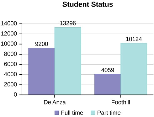
Below are tables comparing the number of part-time and full-time students at De Anza College and Foothill College enrolled for the spring 2010 quarter. The tables display counts (frequencies) and percentages or proportions (relative frequencies). The percent columns make comparing the same categories in the colleges easier. Displaying percentages along with the numbers is often helpful, but it is particularly important when comparing sets of data that do not have the same totals, such as the total enrollments for both colleges in this example. Notice how much larger the percentage for part-time students at Foothill College is compared to De Anza College.

Table 1.2 Fall Term 2007 (Census day)

Tables are a good way of organizing and displaying data. But graphs can be even more helpful in understanding the data. There are no strict rules concerning which graphs to use. Two graphs that are used to display qualitative(categorical) data are pie charts and bar graphs.

In a pie chart, categories of data are represented by wedges in a circle and are proportional in size to the percent of individuals in each category.

In a bar graph, the length of the bar for each category is proportional to the number or percent of individuals in each category. Bars may be vertical or horizontal.

A Pareto chart consists of bars that are sorted into order by category size (largest to smallest).

Look at Figure 1.4 and Figure 1.5 and determine which graph (pie or bar) you think displays the comparisons better.

This OpenStax book is available for free at http://cnx.org/content/col11776/1.33

It is a good idea to look at a variety of graphs to see which is the most helpful in displaying the data. We might make different choices of what we think is the “best” graph depending on the data and the context. Our choice also depends on what we are using the data for.

• (b)

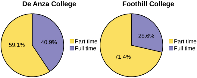
Figure 1.4

Figure 1.5

Percentages That Add to More (or Less) Than 100%

Sometimes percentages add up to be more than 100% (or less than 100%). In the graph, the percentages add to more than 100% because students can be in more than one category. A bar graph is appropriate to compare the relative size of the categories. A pie chart cannot be used. It also could not be used if the percentages added to less than 100%.

Table 1.3 De Anza College Spring 2010

Table 1.3 De Anza College Spring 2010

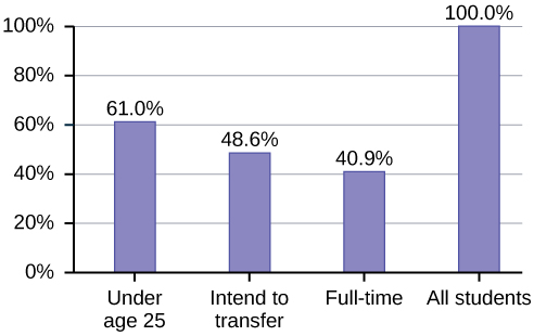
Figure 1.6

Omitting Categories/Missing Data

The table displays Ethnicity of Students but is missing the “Other/Unknown” category. This category contains people who did not feel they fit into any of the ethnicity categories or declined to respond. Notice that the frequencies do not add up to the total number of students. In this situation, create a bar graph and not a pie chart.

Table 1.4 Ethnicity of Students at De Anza College Fall Term 2007 (Census Day)

This OpenStax book is available for free at http://cnx.org/content/col11776/1.33

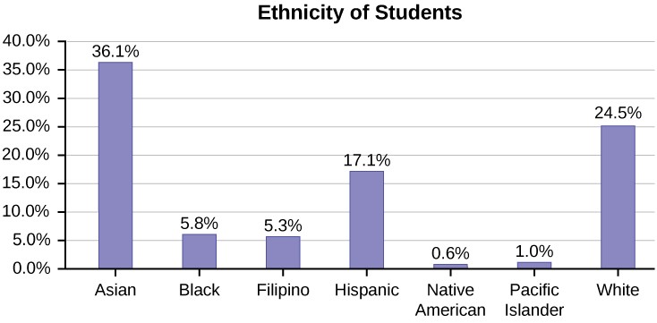
Figure 1.7

The following graph is the same as the previous graph but the “Other/Unknown” percent (9.6%) has been included. The “Other/Unknown” category is large compared to some of the other categories (Native American, 0.6%, Pacific Islander 1.0%). This is important to know when we think about what the data are telling us.

This particular bar graph in Figure 1.8 can be difficult to understand visually. The graph in Figure 1.9 is a Pareto chart. The Pareto chart has the bars sorted from largest to smallest and is easier to read and interpret.

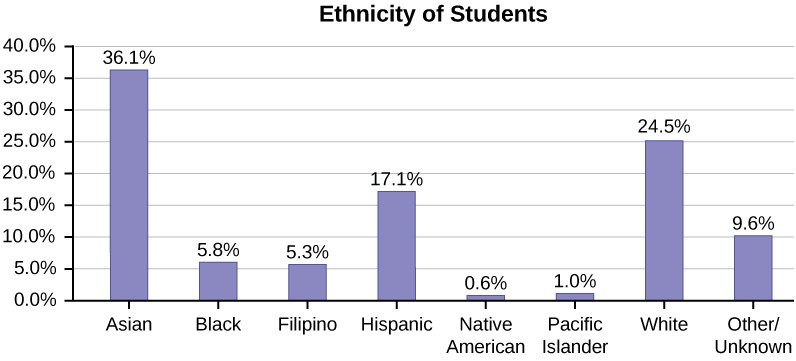
Figure 1.8 Bar Graph with Other/Unknown Category

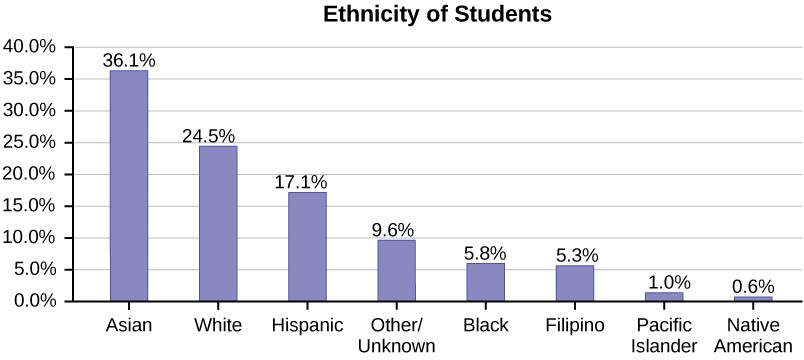
Figure 1.9 Pareto Chart With Bars Sorted by Size

Pie Charts: No Missing Data

The following pie charts have the “Other/Unknown” category included (since the percentages must add to 100%). The chart in Figure 1.10b is organized by the size of each wedge, which makes it a more visually informative graph than the unsorted, alphabetical graph in Figure 1.10a.

Figure 1.10

Sampling

(a)

Gathering information about an entire population often costs too much or is virtually impossible. Instead, we use a sample of the population. A sample should have the same characteristics as the population it is representing. Most statisticians use various methods of random sampling in an attempt to achieve this goal. This section will describe a few of the most common methods. There are several different methods of random sampling. In each form of random sampling, each member of a population initially has an equal chance of being selected for the sample. Each method has pros and cons. The easiest method to describe is called a simple random sample. Any group of n individuals is equally likely to be chosen as any other group of n individuals if the simple random sampling technique is used. In other words, each sample of the same size has an equal chance of being selected.

Besides simple random sampling, there are other forms of sampling that involve a chance process for getting the sample. Other well-known random sampling methods are the stratified sample, the cluster sample, and the systematic sample.

To choose a stratified sample, divide the population into groups called strata and then take a proportionate number from each stratum. For example, you could stratify (group) your college population by department and then choose a

This OpenStax book is available for free at http://cnx.org/content/col11776/1.33

proportionate simple random sample from each stratum (each department) to get a stratified random sample. To choose a simple random sample from each department, number each member of the first department, number each member of the second department, and do the same for the remaining departments. Then use simple random sampling to choose proportionate numbers from the first department and do the same for each of the remaining departments. Those numbers picked from the first department, picked from the second department, and so on represent the members who make up the stratified sample.

To choose a cluster sample, divide the population into clusters (groups) and then randomly select some of the clusters. All the members from these clusters are in the cluster sample. For example, if you randomly sample four departments from your college population, the four departments make up the cluster sample. Divide your college faculty by department. The departments are the clusters. Number each department, and then choose four different numbers using simple random sampling. All members of the four departments with those numbers are the cluster sample.

To choose a systematic sample, randomly select a starting point and take every nth piece of data from a listing of the population. For example, suppose you have to do a phone survey. Your phone book contains 20,000 residence listings. You must choose 400 names for the sample. Number the population 1–20,000 and then use a simple random sample to pick a number that represents the first name in the sample. Then choose every fiftieth name thereafter until you have a total of 400 names (you might have to go back to the beginning of your phone list). Systematic sampling is frequently chosen because it is a simple method.

A type of sampling that is non-random is convenience sampling. Convenience sampling involves using results that are readily available. For example, a computer software store conducts a marketing study by interviewing potential customers who happen to be in the store browsing through the available software. The results of convenience sampling may be very good in some cases and highly biased (favor certain outcomes) in others.

Sampling data should be done very carefully. Collecting data carelessly can have devastating results. Surveys mailed to households and then returned may be very biased (they may favor a certain group). It is better for the person conducting the survey to select the sample respondents.

True random sampling is done with replacement. That is, once a member is picked, that member goes back into the population and thus may be chosen more than once. However for practical reasons, in most populations, simple random sampling is done without replacement. Surveys are typically done without replacement. That is, a member of the population may be chosen only once. Most samples are taken from large populations and the sample tends to be small in comparison to the population. Since this is the case, sampling without replacement is approximately the same as sampling with replacement because the chance of picking the same individual more than once with replacement is very low.

In a college population of 10,000 people, suppose you want to pick a sample of 1,000 randomly for a survey. For any particular sample of 1,000, if you are sampling with replacement,

• the chance of picking the first person is 1,000 out of 10,000 (0.1000);
• the chance of picking a different second person for this sample is 999 out of 10,000 (0.0999);
• the chance of picking the same person again is 1 out of 10,000 (very low). If you are sampling without replacement,
• the chance of picking the first person for any particular sample is 1000 out of 10,000 (0.1000);
• the chance of picking a different second person is 999 out of 9,999 (0.0999);
• you do not replace the first person before picking the next person.

Compare the fractions 999/10,000 and 999/9,999. For accuracy, carry the decimal answers to four decimal places. To four decimal places, these numbers are equivalent (0.0999).

Sampling without replacement instead of sampling with replacement becomes a mathematical issue only when the population is small. For example, if the population is 25 people, the sample is ten, and you are sampling with replacement for any particular sample, then the chance of picking the first person is ten out of 25, and the chance of picking a different second person is nine out of 25 (you replace the first person).

If you sample without replacement, then the chance of picking the first person is ten out of 25, and then the chance of picking the second person (who is different) is nine out of 24 (you do not replace the first person).

Compare the fractions 9/25 and 9/24. To four decimal places, 9/25 = 0.3600 and 9/24 = 0.3750. To four decimal places, these numbers are not equivalent.

When you analyze data, it is important to be aware of sampling errors and nonsampling errors. The actual process of sampling causes sampling errors. For example, the sample may not be large enough. Factors not related to the sampling

process cause nonsampling errors. A defective counting device can cause a nonsampling error.

In reality, a sample will never be exactly representative of the population so there will always be some sampling error. As a rule, the larger the sample, the smaller the sampling error.

In statistics, a sampling bias is created when a sample is collected from a population and some members of the population are not as likely to be chosen as others (remember, each member of the population should have an equally likely chance of being chosen). When a sampling bias happens, there can be incorrect conclusions drawn about the population that is being studied.

Critical Evaluation

We need to evaluate the statistical studies we read about critically and analyze them before accepting the results of the studies. Common problems to be aware of include

• Problems with samples: A sample must be representative of the population. A sample that is not representative of the population is biased. Biased samples that are not representative of the population give results that are inaccurate and not valid.
• Self-selected samples: Responses only by people who choose to respond, such as call-in surveys, are often unreliable.
• Sample size issues: Samples that are too small may be unreliable. Larger samples are better, if possible. In some situations, having small samples is unavoidable and can still be used to draw conclusions. Examples: crash testing cars or medical testing for rare conditions
• Undue influence: collecting data or asking questions in a way that influences the response
• Non-response or refusal of subject to participate: The collected responses may no longer be representative of the population. Often, people with strong positive or negative opinions may answer surveys, which can affect the results.
• Causality: A relationship between two variables does not mean that one causes the other to occur. They may be related (correlated) because of their relationship through a different variable.
• Self-funded or self-interest studies: A study performed by a person or organization in order to support their claim. Is the study impartial? Read the study carefully to evaluate the work. Do not automatically assume that the study is good, but do not automatically assume the study is bad either. Evaluate it on its merits and the work done.
• Misleading use of data: improperly displayed graphs, incomplete data, or lack of context
• Confounding: When the effects of multiple factors on a response cannot be separated. Confounding makes it difficult or impossible to draw valid conclusions about the effect of each factor.

Example 1.11A study is done to determine the average tuition that San Jose State undergraduate students pay per semester. Each student in the following samples is asked how much tuition he or she paid for the Fall semester. What is the type of sampling in each case?A sample of 100 undergraduate San Jose State students is taken by organizing the students’ names by classification (freshman, sophomore, junior, or senior), and then selecting 25 students from each.A random number generator is used to select a student from the alphabetical listing of all undergraduate students in the Fall semester. Starting with that student, every 50th student is chosen until 75 students are included in the sample.A completely random method is used to select 75 students. Each undergraduate student in the fall semester has the same probability of being chosen at any stage of the sampling process.The freshman, sophomore, junior, and senior years are numbered one, two, three, and four, respectively. A random number generator is used to pick two of those years. All students in those two years are in the sample.An administrative assistant is asked to stand in front of the library one Wednesday and to ask the first 100 undergraduate students he encounters what they paid for tuition the Fall semester. Those 100 students are the sample.

This OpenStax book is available for free at http://cnx.org/content/col11776/1.33

Solution 1.11

• stratified; b. systematic; c. simple random; d. cluster; e. convenience

Example 1.12Determine the type of sampling used (simple random, stratified, systematic, cluster, or convenience).A soccer coach selects six players from a group of boys aged eight to ten, seven players from a group of boys aged 11 to 12, and three players from a group of boys aged 13 to 14 to form a recreational soccer team.A pollster interviews all human resource personnel in five different high tech companies.A high school educational researcher interviews 50 high school female teachers and 50 high school male teachers.A medical researcher interviews every third cancer patient from a list of cancer patients at a local hospital.A high school counselor uses a computer to generate 50 random numbers and then picks students whose names correspond to the numbers.A student interviews classmates in his algebra class to determine how many pairs of jeans a student owns, on the average.Solution 1.12a. stratified; b. cluster; c. stratified; d. systematic; e. simple random; f.convenience

If we were to examine two samples representing the same population, even if we used random sampling methods for the samples, they would not be exactly the same. Just as there is variation in data, there is variation in samples. As you become accustomed to sampling, the variability will begin to seem natural.

Example 1.13

Suppose ABC College has 10,000 part-time students (the population). We are interested in the average amount of money a part-time student spends on books in the fall term. Asking all 10,000 students is an almost impossible task.

Suppose we take two different samples.

First, we use convenience sampling and survey ten students from a first term organic chemistry class. Many of these students are taking first term calculus in addition to the organic chemistry class. The amount of money they spend on books is as follows:

$128; $87; $173; $116; $130; $204; $147; $189; $93; $153

The second sample is taken using a list of senior citizens who take P.E. classes and taking every fifth senior citizen on the list, for a total of ten senior citizens. They spend:

$50; $40; $36; $15; $50; $100; $40; $53; $22; $22

It is unlikely that any student is in both samples.

a. Do you think that either of these samples is representative of (or is characteristic of) the entire 10,000 part-time student population?

Solution 1.13

• No. The first sample probably consists of science-oriented students. Besides the chemistry course, some of them are also taking first-term calculus. Books for these classes tend to be expensive. Most of these students are, more than likely, paying more than the average part-time student for their books. The second sample is a group of senior citizens who are, more than likely, taking courses for health and interest. The amount of money they spend on books is probably much less than the average parttime student. Both samples are biased. Also, in both cases,

not all students have a chance to be in either sample.

• Since these samples are not representative of the entire population, is it wise to use the results to describe the entire population?

Solution 1.13

• No. For these samples, each member of the population did not have an equally likely chance of being chosen.

Now, suppose we take a third sample. We choose ten different part-time students from the disciplines of chemistry, math, English, psychology, sociology, history, nursing, physical education, art, and early childhood development. (We assume that these are the only disciplines in which part-time students at ABC College are enrolled and that an equal number of part-time students are enrolled in each of the disciplines.) Each student is chosen using simple random sampling. Using a calculator, random numbers are generated and a student from a particular discipline is selected if he or she has a corresponding number. The students spend the following amounts:

$180; $50; $150; $85; $260; $75; $180; $200; $200; $150

• Is the sample biased?

Solution 1.13

c. The sample is unbiased, but a larger sample would be recommended to increase the likelihood that the sample will be close to representative of the population. However, for a biased sampling technique, even a large sample runs the risk of not being representative of the population.

Students often ask if it is “good enough” to take a sample, instead of surveying the entire population. If the survey is done well, the answer is yes.

1.13 A local radio station has a fan base of 20,000 listeners. The station wants to know if its audience would prefer more music or more talk shows. Asking all 20,000 listeners is an almost impossible task.The station uses convenience sampling and surveys the first 200 people they meet at one of the station’s music concert events. 24 people said they’d prefer more talk shows, and 176 people said they’d prefer more music.Do you think that this sample is representative of (or is characteristic of) the entire 20,000 listener population?

Variation in Data

Variation is present in any set of data. For example, 16-ounce cans of beverage may contain more or less than 16 ounces of liquid. In one study, eight 16 ounce cans were measured and produced the following amount (in ounces) of beverage:

15.8; 16.1; 15.2; 14.8; 15.8; 15.9; 16.0; 15.5

Measurements of the amount of beverage in a 16-ounce can may vary because different people make the measurements or because the exact amount, 16 ounces of liquid, was not put into the cans. Manufacturers regularly run tests to determine if the amount of beverage in a 16-ounce can falls within the desired range.

Be aware that as you take data, your data may vary somewhat from the data someone else is taking for the same purpose. This is completely natural. However, if two or more of you are taking the same data and get very different results, it is time for you and the others to reevaluate your data-taking methods and your accuracy.

Variation in Samples

It was mentioned previously that two or more samples from the same population, taken randomly, and having close to the same characteristics of the population will likely be different from each other. Suppose Doreen and Jung both decide to study the average amount of time students at their college sleep each night. Doreen and Jung each take samples of 500 students. Doreen uses systematic sampling and Jung uses cluster sampling. Doreen’s sample will be different from Jung’s sample. Even if Doreen and Jung used the same sampling method, in all likelihood their samples would be different. Neither

This OpenStax book is available for free at http://cnx.org/content/col11776/1.33

would be wrong, however.

Think about what contributes to making Doreen’s and Jung’s samples different.

If Doreen and Jung took larger samples (i.e. the number of data values is increased), their sample results (the average amount of time a student sleeps) might be closer to the actual population average. But still, their samples would be, in all likelihood, different from each other. This variability in samples cannot be stressed enough.

Size of a Sample

The size of a sample (often called the number of observations, usually given the symbol n) is important. The examples you have seen in this book so far have been small. Samples of only a few hundred observations, or even smaller, are sufficient for many purposes. In polling, samples that are from 1,200 to 1,500 observations are considered large enough and good enough if the survey is random and is well done. Later we will find that even much smaller sample sizes will give very good results. You will learn why when you study confidence intervals.

Be aware that many large samples are biased. For example, call-in surveys are invariably biased, because people choose to respond or not.

| Levels of Measurement

Once you have a set of data, you will need to organize it so that you can analyze how frequently each datum occurs in the set. However, when calculating the frequency, you may need to round your answers so that they are as precise as possible.

Levels of Measurement

The way a set of data is measured is called its level of measurement. Correct statistical procedures depend on a researcher being familiar with levels of measurement. Not every statistical operation can be used with every set of data. Data can be classified into four levels of measurement. They are (from lowest to highest level):

Nominal scale level

• Ordinal scale level
• Interval scale level
• Ratio scale level

Data that is measured using a nominal scale is qualitative (categorical). Categories, colors, names, labels and favorite foods along with yes or no responses are examples of nominal level data. Nominal scale data are not ordered. For example, trying to classify people according to their favorite food does not make any sense. Putting pizza first and sushi second is not meaningful.

Smartphone companies are another example of nominal scale data. The data are the names of the companies that make smartphones, but there is no agreed upon order of these brands, even though people may have personal preferences. Nominal scale data cannot be used in calculations.

Data that is measured using an ordinal scale is similar to nominal scale data but there is a big difference. The ordinal scale data can be ordered. An example of ordinal scale data is a list of the top five national parks in the United States. The top five national parks in the United States can be ranked from one to five but we cannot measure differences between the data.

Another example of using the ordinal scale is a cruise survey where the responses to questions about the cruise are “excellent,” “good,” “satisfactory,” and “unsatisfactory.” These responses are ordered from the most desired response to the least desired. But the differences between two pieces of data cannot be measured. Like the nominal scale data, ordinal scale data cannot be used in calculations.

Data that is measured using the interval scale is similar to ordinal level data because it has a definite ordering but there is a difference between data. The differences between interval scale data can be measured though the data does not have a starting point.

Temperature scales like Celsius (C) and Fahrenheit (F) are measured by using the interval scale. In both temperature measurements, 40° is equal to 100° minus 60°. Differences make sense. But 0 degrees does not because, in both scales, 0 is not the absolute lowest temperature. Temperatures like -10° F and -15° C exist and are colder than 0.

Interval level data can be used in calculations, but one type of comparison cannot be done. 80° C is not four times as hot as 20° C (nor is 80° F four times as hot as 20° F). There is no meaning to the ratio of 80 to 20 (or four to one).

Data that is measured using the ratio scale takes care of the ratio problem and gives you the most information. Ratio scale data is like interval scale data, but it has a 0 point and ratios can be calculated. For example, four multiple choice statistics

final exam scores are 80, 68, 20 and 92 (out of a possible 100 points). The exams are machine-graded. The data can be put in order from lowest to highest: 20, 68, 80, 92.

The differences between the data have meaning. The score 92 is more than the score 68 by 24 points. Ratios can be calculated. The smallest score is 0. So 80 is four times 20. The score of 80 is four times better than the score of 20.

Frequency

Twenty students were asked how many hours they worked per day. Their responses, in hours, are as follows: 5; 6; 3; 3; 2; 4; 7; 5; 2; 3; 5; 6; 5; 4; 4; 3; 5; 2; 5; 3.

Table 1.5 lists the different data values in ascending order and their frequencies.

Table 1.5 Frequency Table of Student Work Hours

A frequency is the number of times a value of the data occurs. According to Table 1.5, there are three students who work two hours, five students who work three hours, and so on. The sum of the values in the frequency column, 20, represents the total number of students included in the sample.

A relative frequency is the ratio (fraction or proportion) of the number of times a value of the data occurs in the set of all outcomes to the total number of outcomes. To find the relative frequencies, divide each frequency by the total number of students in the sample–in this case, 20. Relative frequencies can be written as fractions, percents, or decimals.

Table 1.6 Frequency Table of Student Work Hours with Relative Frequencies

The sum of the values in the relative frequency column of Table 1.6 is 20

20

, or 1.

Cumulative relative frequency is the accumulation of the previous relative frequencies. To find the cumulative relative

This OpenStax book is available for free at http://cnx.org/content/col11776/1.33

frequencies, add all the previous relative frequencies to the relative frequency for the current row, as shown in Table 1.7.

Table 1.7 Frequency Table of Student Work Hours with Relative and Cumulative Relative Frequencies

NOTEBecause of rounding, the relative frequency column may not always sum to one, and the last entry in the cumulative relative frequency column may not be one. However, they each should be close to one.
The last entry of the cumulative relative frequency column is one, indicating that one hundred percent of the data has been accumulated.

Table 1.8 represents the heights, in inches, of a sample of 100 male semiprofessional soccer players.

Table 1.8 Frequency Table of Soccer Player Height

Table 1.8 Frequency Table of Soccer Player Height

The data in this table have been grouped into the following intervals:

• 59.95 to 61.95 inches

• 61.95 to 63.95 inches

• 63.95 to 65.95 inches

• 65.95 to 67.95 inches

• 67.95 to 69.95 inches

• 69.95 to 71.95 inches

• 71.95 to 73.95 inches

• 73.95 to 75.95 inches

In this sample, there are five players whose heights fall within the interval 59.95–61.95 inches, three players whose heights fall within the interval 61.95–63.95 inches, 15 players whose heights fall within the interval 63.95–65.95 inches, 40 players whose heights fall within the interval 65.95–67.95 inches, 17 players whose heights fall within the interval 67.95–69.95 inches, 12 players whose heights fall within the interval 69.95–71.95, seven players whose heights fall within the interval 71.95–73.95, and one player whose heights fall within the interval 73.95–75.95. All heights fall between the endpoints of an interval and not at the endpoints.

Example 1.14From Table 1.8, find the percentage of heights that are less than 65.95 inches.Solution 1.14If you look at the first, second, and third rows, the heights are all less than 65.95 inches. There are 5 + 3 + 15 = 23players whose heights are less than 65.95 inches. The percentage of heights less than 65.95 inches is then 23100or 23%. This percentage is the cumulative relative frequency entry in the third row.

This OpenStax book is available for free at http://cnx.org/content/col11776/1.33

1.14 Table 1.9 shows the amount, in inches, of annual rainfall in a sample of towns.Table 1.9From Table 1.9, find the percentage of rainfall that is less than 9.01 inches.

Example 1.15From Table 1.8, find the percentage of heights that fall between 61.95 and 65.95 inches.Solution 1.15Add the relative frequencies in the second and third rows: 0.03 + 0.15 = 0.18 or 18%.
1.15 From Table 1.9, find the percentage of rainfall that is between 6.99 and 13.05 inches.
Example 1.16Use the heights of the 100 male semiprofessional soccer players in Table 1.8. Fill in the blanks and check your answers.The percentage of heights that are from 67.95 to 71.95 inches is: .The percentage of heights that are from 67.95 to 73.95 inches is: .The percentage of heights that are more than 65.95 inches is: .The number of players in the sample who are between 61.95 and 71.95 inches tall is: .What kind of data are the heights?

f. Describe how you could gather this data (the heights) so that the data are characteristic of all male semiprofessional soccer players.

Remember, you count frequencies. To find the relative frequency, divide the frequency by the total number of data values. To find the cumulative relative frequency, add all of the previous relative frequencies to the relative frequency for the current row.

Solution 1.16

a. 29%

b. 36%

c. 77%

• 87
• quantitative continuous
• Example 1.17Nineteen people were asked how many miles, to the nearest mile, they commute to work each day. The data are as follows: 2; 5; 7; 3; 2; 10; 18; 15; 20; 7; 10; 18; 5; 12; 13; 12; 4; 5; 10. Table 1.10 was produced:Table 1.10 Frequency of Commuting Distancesa. Is the table correct? If it is not correct, what is wrong?
  get rosters from each team and choose a simple random sample from each

This OpenStax book is available for free at http://cnx.org/content/col11776/1.33

• True or False: Three percent of the people surveyed commute three miles. If the statement is not correct, what should it be? If the table is incorrect, make the corrections.
• What fraction of the people surveyed commute five or seven miles?
• What fraction of the people surveyed commute 12 miles or more? Less than 12 miles? Between five and 13 miles (not including five and 13 miles)?

Solution 1.17

• No. The frequency column sums to 18, not 19. Not all cumulative relative frequencies are correct.
• False. The frequency for three miles should be one; for two miles (left out), two. The cumulative relative frequency column should read: 0.1052, 0.1579, 0.2105, 0.3684, 0.4737, 0.6316, 0.7368, 0.7895, 0.8421, 0.9474, 1.0000.

5 19

d. 7 , 12 , 7

191919

1.17 Table 1.9 represents the amount, in inches, of annual rainfall in a sample of towns. What fraction of towns surveyed get between 11.03 and 13.05 inches of rainfall each year?

Example 1.18

Table 1.11 contains the total number of deaths worldwide as a result of earthquakes for the period from 2000 to 2012.

Table 1.11

Answer the following questions.

• What is the frequency of deaths measured from 2006 through 2009?
• What percentage of deaths occurred after 2009?
• What is the relative frequency of deaths that occurred in 2003 or earlier?
• What is the percentage of deaths that occurred in 2004?
• What kind of data are the numbers of deaths?
• The Richter scale is used to quantify the energy produced by an earthquake. Examples of Richter scale numbers are 2.3, 4.0, 6.1, and 7.0. What kind of data are these numbers?

Solution 1.18

a. 97,118 (11.8%)

b. 41.6%

c. 67,092/823,356 or 0.081 or 8.1 % d. 27.8%

• Quantitative discrete
• Quantitative continuous

This OpenStax book is available for free at http://cnx.org/content/col11776/1.33

1.18 Table 1.12 contains the total number of fatal motor vehicle traffic crashes in the United States for the period from 1994 to 2011.Table 1.12Answer the following questions.What is the frequency of deaths measured from 2000 through 2004?What percentage of deaths occurred after 2006?What is the relative frequency of deaths that occurred in 2000 or before?What is the percentage of deaths that occurred in 2011?What is the cumulative relative frequency for 2006? Explain what this number tells you about the data.
| Experimental Design and Ethics

Does aspirin reduce the risk of heart attacks? Is one brand of fertilizer more effective at growing roses than another? Is fatigue as dangerous to a driver as the influence of alcohol? Questions like these are answered using randomized experiments. In this module, you will learn important aspects of experimental design. Proper study design ensures the production of reliable, accurate data.

The purpose of an experiment is to investigate the relationship between two variables. When one variable causes change in another, we call the first variable the independent variable or explanatory variable. The affected variable is called the dependent variable or response variable: stimulus, response. In a randomized experiment, the researcher manipulates values of the explanatory variable and measures the resulting changes in the response variable. The different values of the explanatory variable are called treatments. An experimental unit is a single object or individual to be measured.

You want to investigate the effectiveness of vitamin E in preventing disease. You recruit a group of subjects and ask them if they regularly take vitamin E. You notice that the subjects who take vitamin E exhibit better health on average than those who do not. Does this prove that vitamin E is effective in disease prevention? It does not. There are many differences between the two groups compared in addition to vitamin E consumption. People who take vitamin E regularly often take other steps to improve their health: exercise, diet, other vitamin supplements, choosing not to smoke. Any one of these factors could be influencing health. As described, this study does not prove that vitamin E is the key to disease prevention.

Additional variables that can cloud a study are called lurking variables. In order to prove that the explanatory variable is causing a change in the response variable, it is necessary to isolate the explanatory variable. The researcher must design her experiment in such a way that there is only one difference between groups being compared: the planned treatments. This is

accomplished by the random assignment of experimental units to treatment groups. When subjects are assigned treatments randomly, all of the potential lurking variables are spread equally among the groups. At this point the only difference between groups is the one imposed by the researcher. Different outcomes measured in the response variable, therefore, must be a direct result of the different treatments. In this way, an experiment can prove a cause-and-effect connection between the explanatory and response variables.

The power of suggestion can have an important influence on the outcome of an experiment. Studies have shown that the expectation of the study participant can be as important as the actual medication. In one study of performance-enhancing drugs, researchers noted:

Results showed that believing one had taken the substance resulted in [performance] times almost as fast as those associated with consuming the drug itself. In contrast, taking the drug without knowledge yielded no significant performance increment.[1]

When participation in a study prompts a physical response from a participant, it is difficult to isolate the effects of the explanatory variable. To counter the power of suggestion, researchers set aside one treatment group as a control group. This group is given a placebo treatment–a treatment that cannot influence the response variable. The control group helps researchers balance the effects of being in an experiment with the effects of the active treatments. Of course, if you are participating in a study and you know that you are receiving a pill which contains no actual medication, then the power of suggestion is no longer a factor. Blinding in a randomized experiment preserves the power of suggestion. When a person involved in a research study is blinded, he does not know who is receiving the active treatment(s) and who is receiving the placebo treatment. A double-blind experiment is one in which both the subjects and the researchers involved with the subjects are blinded.

Example 1.19The Smell & Taste Treatment and Research Foundation conducted a study to investigate whether smell can affect learning. Subjects completed mazes multiple times while wearing masks. They completed the pencil and paper mazes three times wearing floral-scented masks, and three times with unscented masks. Participants were assigned at random to wear the floral mask during the first three trials or during the last three trials. For each trial, researchers recorded the time it took to complete the maze and the subject’s impression of the mask’s scent: positive, negative, or neutral.Describe the explanatory and response variables in this study.What are the treatments?Identify any lurking variables that could interfere with this study.Is it possible to use blinding in this study?Solution 1.19The explanatory variable is scent, and the response variable is the time it takes to complete the maze.There are two treatments: a floral-scented mask and an unscented mask.All subjects experienced both treatments. The order of treatments was randomly assigned so there were no differences between the treatment groups. Random assignment eliminates the problem of lurking variables.Subjects will clearly know whether they can smell flowers or not, so subjects cannot be blinded in this study. Researchers timing the mazes can be blinded, though. The researcher who is observing a subject will not know which mask is being worn.

• McClung, M. Collins, D. “Because I know it will!”: placebo effects of an ergogenic aid on athletic performance. Journal of Sport & Exercise Psychology. 2007 Jun. 29(3):382-94. Web. April 30, 2013.

This OpenStax book is available for free at http://cnx.org/content/col11776/1.33

KEY TERMS

Average also called mean or arithmetic mean; a number that describes the central tendency of the data

Blinding not telling participants which treatment a subject is receiving

Categorical Variable variables that take on values that are names or labels

Cluster Sampling a method for selecting a random sample and dividing the population into groups (clusters); use simple random sampling to select a set of clusters. Every individual in the chosen clusters is included in the sample.

Continuous Random Variable a random variable (RV) whose outcomes are measured; the height of trees in the forest is a continuous RV.

Control Group a group in a randomized experiment that receives an inactive treatment but is otherwise managed exactly as the other groups

Convenience Sampling a nonrandom method of selecting a sample; this method selects individuals that are easily accessible and may result in biased data.

Cumulative Relative Frequency The term applies to an ordered set of observations from smallest to largest. The cumulative relative frequency is the sum of the relative frequencies for all values that are less than or equal to the given value.

Data a set of observations (a set of possible outcomes); most data can be put into two groups: qualitative (an attribute whose value is indicated by a label) or quantitative (an attribute whose value is indicated by a number). Quantitative data can be separated into two subgroups: discrete and continuous. Data is discrete if it is the result of counting (such as the number of students of a given ethnic group in a class or the number of books on a shelf). Data is continuous if it is the result of measuring (such as distance traveled or weight of luggage)

Discrete Random Variable a random variable (RV) whose outcomes are counted

Double-blinding the act of blinding both the subjects of an experiment and the researchers who work with the subjects

Experimental Unit any individual or object to be measured

Explanatory Variable the independent variable in an experiment; the value controlled by researchers

Frequency the number of times a value of the data occurs

Informed Consent Any human subject in a research study must be cognizant of any risks or costs associated with the study. The subject has the right to know the nature of the treatments included in the study, their potential risks, and their potential benefits. Consent must be given freely by an informed, fit participant.

Institutional Review Board a committee tasked with oversight of research programs that involve human subjects

Lurking Variable a variable that has an effect on a study even though it is neither an explanatory variable nor a response variable

Mathematical Models a description of a phenomenon using mathematical concepts, such as equations, inequalities, distributions, etc.

Nonsampling Error an issue that affects the reliability of sampling data other than natural variation; it includes a variety of human errors including poor study design, biased sampling methods, inaccurate information provided by study participants, data entry errors, and poor analysis.

Numerical Variable variables that take on values that are indicated by numbers

Observational Study a study in which the independent variable is not manipulated by the researcher

Parameter a number that is used to represent a population characteristic and that generally cannot be determined easily

Placebo an inactive treatment that has no real effect on the explanatory variable

Population all individuals, objects, or measurements whose properties are being studied

Probability a number between zero and one, inclusive, that gives the likelihood that a specific event will occur

Proportion the number of successes divided by the total number in the sample

Qualitative Data See Data. Quantitative Data See Data.

Random Assignment the act of organizing experimental units into treatment groups using random methods

Random Sampling a method of selecting a sample that gives every member of the population an equal chance of being selected.

Relative Frequency the ratio of the number of times a value of the data occurs in the set of all outcomes to the number of all outcomes to the total number of outcomes

Representative Sample a subset of the population that has the same characteristics as the population

Response Variable the dependent variable in an experiment; the value that is measured for change at the end of an experiment

Sample a subset of the population studied

Sampling Bias not all members of the population are equally likely to be selected

Sampling Error the natural variation that results from selecting a sample to represent a larger population; this variation decreases as the sample size increases, so selecting larger samples reduces sampling error.

Sampling with Replacement Once a member of the population is selected for inclusion in a sample, that member is returned to the population for the selection of the next individual.

Sampling without Replacement A member of the population may be chosen for inclusion in a sample only once. If chosen, the member is not returned to the population before the next selection.

Simple Random Sampling a straightforward method for selecting a random sample; give each member of the population a number. Use a random number generator to select a set of labels. These randomly selected labels identify the members of your sample.

Statistic a numerical characteristic of the sample; a statistic estimates the corresponding population parameter.

Statistical Models a description of a phenomenon using probability distributions that describe the expected behavior of the phenomenon and the variability in the expected observations.

Stratified Sampling a method for selecting a random sample used to ensure that subgroups of the population are represented adequately; divide the population into groups (strata). Use simple random sampling to identify a proportionate number of individuals from each stratum.

Survey a study in which data is collected as reported by individuals.

Systematic Sampling a method for selecting a random sample; list the members of the population. Use simple random sampling to select a starting point in the population. Let k = (number of individuals in the population)/(number of individuals needed in the sample). Choose every kth individual in the list starting with the one that was randomly selected. If necessary, return to the beginning of the population list to complete your sample.

Treatments different values or components of the explanatory variable applied in an experiment

Variable a characteristic of interest for each person or object in a population

This OpenStax book is available for free at http://cnx.org/content/col11776/1.33

CHAPTER REVIEW

Definitions of Statistics, Probability, and Key Terms

The mathematical theory of statistics is easier to learn when you know the language. This module presents important terms that will be used throughout the text.

Data, Sampling, and Variation in Data and Sampling

Data are individual items of information that come from a population or sample. Data may be classified as qualitative (categorical), quantitative continuous, or quantitative discrete.

Because it is not practical to measure the entire population in a study, researchers use samples to represent the population. A random sample is a representative group from the population chosen by using a method that gives each individual in the population an equal chance of being included in the sample. Random sampling methods include simple random sampling, stratified sampling, cluster sampling, and systematic sampling. Convenience sampling is a nonrandom method of choosing a sample that often produces biased data.

Samples that contain different individuals result in different data. This is true even when the samples are well-chosen and representative of the population. When properly selected, larger samples model the population more closely than smaller samples. There are many different potential problems that can affect the reliability of a sample. Statistical data needs to be critically analyzed, not simply accepted.

Levels of Measurement

Some calculations generate numbers that are artificially precise. It is not necessary to report a value to eight decimal places when the measures that generated that value were only accurate to the nearest tenth. Round off your final answer to one more decimal place than was present in the original data. This means that if you have data measured to the nearest tenth of a unit, report the final statistic to the nearest hundredth.

In addition to rounding your answers, you can measure your data using the following four levels of measurement.

• Nominal scale level: data that cannot be ordered nor can it be used in calculations
• Ordinal scale level: data that can be ordered; the differences cannot be measured
• Interval scale level: data with a definite ordering but no starting point; the differences can be measured, but there is no such thing as a ratio.
• Ratio scale level: data with a starting point that can be ordered; the differences have meaning and ratios can be calculated.

When organizing data, it is important to know how many times a value appears. How many statistics students study five hours or more for an exam? What percent of families on our block own two pets? Frequency, relative frequency, and cumulative relative frequency are measures that answer questions like these.

Experimental Design and Ethics

A poorly designed study will not produce reliable data. There are certain key components that must be included in every experiment. To eliminate lurking variables, subjects must be assigned randomly to different treatment groups. One of the groups must act as a control group, demonstrating what happens when the active treatment is not applied. Participants in the control group receive a placebo treatment that looks exactly like the active treatments but cannot influence the response variable. To preserve the integrity of the placebo, both researchers and subjects may be blinded. When a study is designed properly, the only difference between treatment groups is the one imposed by the researcher. Therefore, when groups respond differently to different treatments, the difference must be due to the influence of the explanatory variable.

“An ethics problem arises when you are considering an action that benefits you or some cause you support, hurts or reduces benefits to others, and violates some rule.”[2] Ethical violations in statistics are not always easy to spot. Professional associations and federal agencies post guidelines for proper conduct. It is important that you learn basic statistical procedures so that you can recognize proper data analysis.

• Andrew Gelman, “Open Data and Open Methods,” Ethics and Statistics, http://www.stat.columbia.edu/~gelman/ research/published/ChanceEthics1.pdf (accessed May 1, 2013).

HOMEWORK

Definitions of Statistics, Probability, and Key Terms

For each of the following eight exercises, identify: a. the population, b. the sample, c. the parameter, d. the statistic, e. the variable, and f. the data. Give examples where appropriate.

• A fitness center is interested in the mean amount of time a client exercises in the center each week.
• Ski resorts are interested in the mean age that children take their first ski and snowboard lessons. They need this information to plan their ski classes optimally.
• A cardiologist is interested in the mean recovery period of her patients who have had heart attacks.
• Insurance companies are interested in the mean health costs each year of their clients, so that they can determine the costs of health insurance.
• A politician is interested in the proportion of voters in his district who think he is doing a good job.
• A marriage counselor is interested in the proportion of clients she counsels who stay married.
• Political pollsters may be interested in the proportion of people who will vote for a particular cause.
• A marketing company is interested in the proportion of people who will buy a particular product.

Use the following information to answer the next three exercises: A Lake Tahoe Community College instructor is interested in the mean number of days Lake Tahoe Community College math students are absent from class during a quarter.

• What is the population she is interested in?
• all Lake Tahoe Community College students
• all Lake Tahoe Community College English students
• all Lake Tahoe Community College students in her classes
• all Lake Tahoe Community College math students
• Consider the following:

X = number of days a Lake Tahoe Community College math student is absent In this case, X is an example of a:

• variable.
• population.
• statistic.
• data.
• The instructor’s sample produces a mean number of days absent of 3.5 days. This value is an example of a:
• parameter.
• data.
• statistic.
• variable.

Data, Sampling, and Variation in Data and Sampling

For the following exercises, identify the type of data that would be used to describe a response (quantitative discrete, quantitative continuous, or qualitative), and give an example of the data.

• number of tickets sold to a concert
• percent of body fat
• favorite baseball team
• time in line to buy groceries
• number of students enrolled at Evergreen Valley College
• most-watched television show
• brand of toothpaste

This OpenStax book is available for free at http://cnx.org/content/col11776/1.33

• distance to the closest movie theatre
• age of executives in Fortune 500 companies
• number of competing computer spreadsheet software packages

Use the following information to answer the next two exercises: A study was done to determine the age, number of times per week, and the duration (amount of time) of resident use of a local park in San Jose. The first house in the neighborhood around the park was selected randomly and then every 8th house in the neighborhood around the park was interviewed.

• “Number of times per week” is what type of data?
• qualitative (categorical)
• quantitative discrete
• quantitative continuous
• “Duration (amount of time)” is what type of data?
• qualitative (categorical)
• quantitative discrete
• quantitative continuous
• Airline companies are interested in the consistency of the number of babies on each flight, so that they have adequate safety equipment. Suppose an airline conducts a survey. Over Thanksgiving weekend, it surveys six flights from Boston to Salt Lake City to determine the number of babies on the flights. It determines the amount of safety equipment needed by the result of that study.
• Using complete sentences, list three things wrong with the way the survey was conducted.
• Using complete sentences, list three ways that you would improve the survey if it were to be repeated.
• Suppose you want to determine the mean number of students per statistics class in your state. Describe a possible sampling method in three to five complete sentences. Make the description detailed.
• Suppose you want to determine the mean number of cans of soda drunk each month by students in their twenties at your school. Describe a possible sampling method in three to five complete sentences. Make the description detailed.
• List some practical difficulties involved in getting accurate results from a telephone survey.
• List some practical difficulties involved in getting accurate results from a mailed survey.
• With your classmates, brainstorm some ways you could overcome these problems if you needed to conduct a phone or mail survey.
• The instructor takes her sample by gathering data on five randomly selected students from each Lake Tahoe Community College math class. The type of sampling she used is
• cluster sampling
• stratified sampling
• simple random sampling
• convenience sampling
• A study was done to determine the age, number of times per week, and the duration (amount of time) of residents using a local park in San Jose. The first house in the neighborhood around the park was selected randomly and then every eighth house in the neighborhood around the park was interviewed. The sampling method was:
• simple random
• systematic
• stratified
• cluster

• Name the sampling method used in each of the following situations:
• A woman in the airport is handing out questionnaires to travelers asking them to evaluate the airport’s service. She does not ask travelers who are hurrying through the airport with their hands full of luggage, but instead asks all travelers who are sitting near gates and not taking naps while they wait.
• A teacher wants to know if her students are doing homework, so she randomly selects rows two and five and then calls on all students in row two and all students in row five to present the solutions to homework problems to the class.
• The marketing manager for an electronics chain store wants information about the ages of its customers. Over the next two weeks, at each store location, 100 randomly selected customers are given questionnaires to fill out asking for information about age, as well as about other variables of interest.
• The librarian at a public library wants to determine what proportion of the library users are children. The librarian has a tally sheet on which she marks whether books are checked out by an adult or a child. She records this data for every fourth patron who checks out books.
• A political party wants to know the reaction of voters to a debate between the candidates. The day after the debate, the party’s polling staff calls 1,200 randomly selected phone numbers. If a registered voter answers the phone or is available to come to the phone, that registered voter is asked whom he or she intends to vote for and whether the debate changed his or her opinion of the candidates.
• A “random survey” was conducted of 3,274 people of the “microprocessor generation” (people born since 1971, the year the microprocessor was invented). It was reported that 48% of those individuals surveyed stated that if they had $2,000 to spend, they would use it for computer equipment. Also, 66% of those surveyed considered themselves relatively savvy computer users.
• Do you consider the sample size large enough for a study of this type? Why or why not?
• Based on your “gut feeling,” do you believe the percents accurately reflect the U.S. population for those individuals born since 1971? If not, do you think the percents of the population are actually higher or lower than the sample statistics? Why?

Additional information: The survey, reported by Intel Corporation, was filled out by individuals who visited the Los Angeles Convention Center to see the Smithsonian Institute’s road show called “America’s Smithsonian.”

• With this additional information, do you feel that all demographic and ethnic groups were equally represented at the event? Why or why not?
• With the additional information, comment on how accurately you think the sample statistics reflect the population parameters.
• The Well-Being Index is a survey that follows trends of U.S. residents on a regular basis. There are six areas of health and wellness covered in the survey: Life Evaluation, Emotional Health, Physical Health, Healthy Behavior, Work Environment, and Basic Access. Some of the questions used to measure the Index are listed below.

Identify the type of data obtained from each question used in this survey: qualitative(categorical), quantitative discrete, or quantitative continuous.

• Do you have any health problems that prevent you from doing any of the things people your age can normally do?
• During the past 30 days, for about how many days did poor health keep you from doing your usual activities?
• In the last seven days, on how many days did you exercise for 30 minutes or more?
• Do you have health insurance coverage?
• In advance of the 1936 Presidential Election, a magazine titled Literary Digest released the results of an opinion poll predicting that the republican candidate Alf Landon would win by a large margin. The magazine sent post cards to approximately 10,000,000 prospective voters. These prospective voters were selected from the subscription list of the magazine, from automobile registration lists, from phone lists, and from club membership lists. Approximately 2,300,000 people returned the postcards.
• Think about the state of the United States in 1936. Explain why a sample chosen from magazine subscription lists, automobile registration lists, phone books, and club membership lists was not representative of the population of the United States at that time.
• What effect does the low response rate have on the reliability of the sample?
• Are these problems examples of sampling error or nonsampling error?
• During the same year, George Gallup conducted his own poll of 30,000 prospective voters. These researchers used a method they called “quota sampling” to obtain survey answers from specific subsets of the population. Quota sampling is an example of which sampling method described in this module?

This OpenStax book is available for free at http://cnx.org/content/col11776/1.33

• Crime-related and demographic statistics for 47 US states in 1960 were collected from government agencies, including the FBI’s Uniform Crime Report. One analysis of this data found a strong connection between education and crime indicating that higher levels of education in a community correspond to higher crime rates.

Which of the potential problems with samples discussed in Section 1.2 could explain this connection?

• YouPolls is a website that allows anyone to create and respond to polls. One question posted April 15 asks:

“Do you feel happy paying your taxes when members of the Obama administration are allowed to ignore their tax liabilities?”[3]

As of April 25, 11 people responded to this question. Each participant answered “NO!”

Which of the potential problems with samples discussed in this module could explain this connection?

• A scholarly article about response rates begins with the following quote:

“Declining contact and cooperation rates in random digit dial (RDD) national telephone surveys raise serious concerns about the validity of estimates drawn from such research.”[4]

The Pew Research Center for People and the Press admits:

“The percentage of people we interview – out of all we try to interview – has been declining over the past decade or more.”[5]

• What are some reasons for the decline in response rate over the past decade?
• Explain why researchers are concerned with the impact of the declining response rate on public opinion polls.

Levels of Measurement

• Fifty part-time students were asked how many courses they were taking this term. The (incomplete) results are shown below:

Table 1.13 Part-time Student Course Loads

• Fill in the blanks in Table 1.13.
• What percent of students take exactly two courses?
• What percent of students take one or two courses?

• lastbaldeagle. 2013. On Tax Day, House to Call for Firing Federal Workers Who Owe Back Taxes. Opinion poll posted online at: http://www.youpolls.com/details.aspx?id=12328 (accessed May 1, 2013).
• Scott Keeter et al., “Gauging the Impact of Growing Nonresponse on Estimates from a National RDD Telephone Survey,” Public Opinion Quarterly 70 no. 5 (2006), http://poq.oxfordjournals.org/content/70/5/759.full (http://poq.oxfordjournals.org/content/70/5/759.full) (accessed May 1, 2013).
• Frequently Asked Questions, Pew Research Center for the People & the Press, http://www.people-press.org/ methodology/frequently-asked-questions/#dont-you-have-trouble-getting-people-to-answer-your-polls (accessed May 1, 2013).

• Sixty adults with gum disease were asked the number of times per week they used to floss before their diagnosis. The (incomplete) results are shown in Table 1.14.

Table 1.14 Flossing Frequency for Adults with Gum Disease

• Fill in the blanks in Table 1.14.
• What percent of adults flossed six times per week?
• What percent flossed at most three times per week?
• Nineteen immigrants to the U.S were asked how many years, to the nearest year, they have lived in the U.S. The data are as follows: 2; 5; 7; 2; 2; 10; 20; 15; 0; 7; 0; 20; 5; 12; 15; 12; 4; 5; 10.

Table 1.15 was produced.

Table 1.15 Frequency of Immigrant Survey Responses

• Fix the errors in Table 1.15. Also, explain how someone might have arrived at the incorrect number(s).
• Explain what is wrong with this statement: “47 percent of the people surveyed have lived in the U.S. for 5 years.”
• Fix the statement in b to make it correct.
• What fraction of the people surveyed have lived in the U.S. five or seven years?
• What fraction of the people surveyed have lived in the U.S. at most 12 years?
• What fraction of the people surveyed have lived in the U.S. fewer than 12 years?
• What fraction of the people surveyed have lived in the U.S. from five to 20 years, inclusive?

This OpenStax book is available for free at http://cnx.org/content/col11776/1.33

• How much time does it take to travel to work? Table 1.16 shows the mean commute time by state for workers at least 16 years old who are not working at home. Find the mean travel time, and round off the answer properly.

Table 1.16

• Forbes magazine published data on the best small firms in 2012. These were firms which had been publicly traded for at least a year, have a stock price of at least $5 per share, and have reported annual revenue between $5 million and $1 billion. Table 1.17 shows the ages of the chief executive officers for the first 60 ranked firms.

Table 1.17

• What is the frequency for CEO ages between 54 and 65?
• What percentage of CEOs are 65 years or older?
• What is the relative frequency of ages under 50?
• What is the cumulative relative frequency for CEOs younger than 55?
• Which graph shows the relative frequency and which shows the cumulative relative frequency?

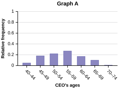
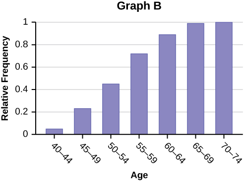
(a)(b)

Figure 1.11

Use the following information to answer the next two exercises: Table 1.18 contains data on hurricanes that have made direct hits on the U.S. Between 1851 and 2004. A hurricane is given a strength category rating based on the minimum wind speed generated by the storm.

Table 1.18 Frequency of Hurricane Direct Hits

• What is the relative frequency of direct hits that were category 4 hurricanes? a. 0.0768

b. 0.0659

c. 0.2601

• Not enough information to calculate
• What is the relative frequency of direct hits that were AT MOST a category 3 storm? a. 0.3480

b. 0.9231

c. 0.2601

d. 0.3370

REFERENCES

Definitions of Statistics, Probability, and Key Terms

The Data and Story Library, http://lib.stat.cmu.edu/DASL/Stories/CrashTestDummies.html (accessed May 1, 2013).

Data, Sampling, and Variation in Data and Sampling

Gallup-Healthways Well-Being Index. http://www.well-beingindex.com/default.asp (accessed May 1, 2013). Gallup-Healthways Well-Being Index. http://www.well-beingindex.com/methodology.asp (accessed May 1, 2013).

Gallup-HealthwaysWell-BeingIndex.http://www.gallup.com/poll/146822/gallup-healthways-index-questions.aspx (accessed May 1, 2013).

Data from http://www.bookofodds.com/Relationships-Society/Articles/A0374-How-George-Gallup-Picked-the-President

Dominic Lusinchi, “’President’ Landon and the 1936 Literary Digest Poll: Were Automobile and Telephone Owners to Blame?” Social Science History 36, no. 1: 23-54 (2012), http://ssh.dukejournals.org/content/36/1/23.abstract (accessed May

1, 2013).

“The Literary Digest Poll,” Virtual Laboratories in Probability and Statistics http://www.math.uah.edu/stat/data/ LiteraryDigest.html (accessed May 1, 2013).

“Gallup Presidential Election Trial-Heat Trends, 1936–2008,” Gallup Politics http://www.gallup.com/poll/110548/gallup- presidential-election-trialheat-trends-19362004.aspx#4 (accessed May 1, 2013).

The Data and Story Library, http://lib.stat.cmu.edu/DASL/Datafiles/USCrime.html (accessed May 1, 2013).

LBCC Distance Learning (DL) program data in 2010-2011, http://de.lbcc.edu/reports/2010-11/future/highlights.html#focus (accessed May 1, 2013).

This OpenStax book is available for free at http://cnx.org/content/col11776/1.33

Data from San Jose Mercury News

Levels of Measurement

“State & County QuickFacts,” U.S. Census Bureau. http://quickfacts.census.gov/qfd/download_data.html (accessed May 1, 2013).

“State & County QuickFacts: Quick, easy access to facts about people, business, and geography,” U.S. Census Bureau. http://quickfacts.census.gov/qfd/index.html (accessed May 1, 2013).

“Table 5: Direct hits by mainland United States Hurricanes (1851-2004),” National Hurricane Center, http://www.nhc.noaa.gov/gifs/table5.gif (accessed May 1, 2013).

“Levels of Measurement,” http://infinity.cos.edu/faculty/woodbury/stats/tutorial/Data_Levels.htm (accessed May 1, 2013).

Courtney Taylor, “Levels of Measurement,” about.com, http://statistics.about.com/od/HelpandTutorials/a/Levels-Of- Measurement.htm (accessed May 1, 2013).

David Lane. “Levels of Measurement,” Connexions, http://cnx.org/content/m10809/latest/ (accessed May 1, 2013).

Experimental Design and Ethics

“Vitamin E and Health,” Nutrition Source, Harvard School of Public Health, http://www.hsph.harvard.edu/nutritionsource/ vitamin-e/ (accessed May 1, 2013).

Stan Reents. “Don’t Underestimate the Power of Suggestion,” athleteinme.com, http://www.athleteinme.com/ ArticleView.aspx?id=1053 (accessed May 1, 2013).

Ankita Mehta. “Daily Dose of Aspiring Helps Reduce Heart Attacks: Study,” International Business Times, July 21, 2011. Also available online at http://www.ibtimes.com/daily-dose-aspirin-helps-reduce-heart-attacks-study-300443 (accessed May 1, 2013).

The Data and Story Library, http://lib.stat.cmu.edu/DASL/Stories/ScentsandLearning.html (accessed May 1, 2013).

M.L. Jacskon et al., “Cognitive Components of Simulated Driving Performance: Sleep Loss effect and Predictors,” Accident Analysis and Prevention Journal, Jan no. 50 (2013), http://www.ncbi.nlm.nih.gov/pubmed/22721550 (accessed May 1, 2013).

“Earthquake Information by Year,” U.S. Geological Survey. http://earthquake.usgs.gov/earthquakes/eqarchives/year/ (accessed May 1, 2013).

“Fatality Analysis Report Systems (FARS) Encyclopedia,” National Highway Traffic and Safety Administration. http://www-fars.nhtsa.dot.gov/Main/index.aspx (accessed May 1, 2013).

Data from www.businessweek.com (accessed May 1, 2013). Data from www.forbes.com (accessed May 1, 2013).

“America’s Best Small Companies,” http://www.forbes.com/best-small-companies/list/ (accessed May 1, 2013).

U.S. Department of Health and Human Services, Code of Federal Regulations Title 45 Public Welfare Department of Health and Human Services Part 46 Protection of Human Subjects revised January 15, 2009. Section 46.111:Criteria for IRB Approval of Research.

“April 2013 Air Travel Consumer Report,” U.S. Department of Transportation, April 11 (2013), http://www.dot.gov/ airconsumer/april-2013-air-travel-consumer-report (accessed May 1, 2013).

Lori Alden, “Statistics can be Misleading,” econoclass.com, http://www.econoclass.com/misleadingstats.html (accessed May 1, 2013).

Maria de los A. Medina, “Ethics in Statistics,” Based on “Building an Ethics Module for Business, Science, and Engineering Students” by Jose A. Cruz-Cruz and William Frey, Connexions, http://cnx.org/content/m15555/latest/ (accessed May 1, 2013).

SOLUTIONS

2

• all children who take ski or snowboard lessons
• a group of these children
• the population mean age of children who take their first snowboard lesson
• the sample mean age of children who take their first snowboard lesson
• X = the age of one child who takes his or her first ski or snowboard lesson
• values for X, such as 3, 7, and so on

4

• the clients of the insurance companies
• a group of the clients
• the mean health costs of the clients
• the mean health costs of the sample
• X = the health costs of one client
• values for X, such as 34, 9, 82, and so on

6

• all the clients of this counselor
• a group of clients of this marriage counselor
• the proportion of all her clients who stay married
• the proportion of the sample of the counselor’s clients who stay married
• X = the number of couples who stay married
• yes, no

8

• all people (maybe in a certain geographic area, such as the United States)
• a group of the people
• the proportion of all people who will buy the product
• the proportion of the sample who will buy the product
• X = the number of people who will buy it
• buy, not buy

10 a

12 quantitative discrete, 150

14 qualitative, Oakland A’s

16 quantitative discrete, 11,234 students

18 qualitative, Crest

20 quantitative continuous, 47.3 years

22 b

24

• The survey was conducted using six similar flights.

The survey would not be a true representation of the entire population of air travelers. Conducting the survey on a holiday weekend will not produce representative results.

• Conduct the survey during different times of the year.

This OpenStax book is available for free at http://cnx.org/content/col11776/1.33

Conduct the survey using flights to and from various locations. Conduct the survey on different days of the week.

26 Answers will vary. Sample Answer: You could use a systematic sampling method. Stop the tenth person as they leave one of the buildings on campus at 9:50 in the morning. Then stop the tenth person as they leave a different building on campus at 1:50 in the afternoon.

28 Answers will vary. Sample Answer: Many people will not respond to mail surveys. If they do respond to the surveys, you can’t be sure who is responding. In addition, mailing lists can be incomplete.

30 b

32 convenience; cluster; stratified ; systematic; simple random

34

• qualitative(categorical)
• quantitative discrete
• quantitative discrete
• qualitative(categorical)

36 Causality: The fact that two variables are related does not guarantee that one variable is influencing the other. We cannot assume that crime rate impacts education level or that education level impacts crime rate. Confounding: There are many factors that define a community other than education level and crime rate. Communities with high crime rates and high education levels may have other lurking variables that distinguish them from communities with lower crime rates and lower education levels. Because we cannot isolate these variables of interest, we cannot draw valid conclusions about the connection between education and crime. Possible lurking variables include police expenditures, unemployment levels, region, average age, and size.

38

• Possible reasons: increased use of caller id, decreased use of landlines, increased use of private numbers, voice mail, privacy managers, hectic nature of personal schedules, decreased willingness to be interviewed
• When a large number of people refuse to participate, then the sample may not have the same characteristics of the population. Perhaps the majority of people willing to participate are doing so because they feel strongly about the subject of the survey.

40

a.

Table 1.19

b. 5.00%

c. 93.33%

42 The sum of the travel times is 1,173.1. Divide the sum by 50 to calculate the mean value: 23.462. Because each state’s travel time was measured to the nearest tenth, round this calculation to the nearest hundredth: 23.46.

44 b

This OpenStax book is available for free at http://cnx.org/content/col11776/1.33