7 7 | THE CENTRAL LIMIT THEOREM

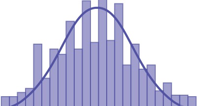
Figure 7.1 If you want to figure out the distribution of the change people carry in their pockets, using the Central Limit Theorem and assuming your sample is large enough, you will find that the distribution is the normal probability density function. (credit: John Lodder)

Introduction

Why are we so concerned with means? Two reasons are: they give us a middle ground for comparison, and they are easy to calculate. In this chapter, you will study means and the Central Limit Theorem.

The Central Limit Theorem is one of the most powerful and useful ideas in all of statistics. The Central Limit Theorem is a theorem which means that it is NOT a theory or just somebody’s idea of the way things work. As a theorem it ranks with the Pythagorean Theorem, or the theorem that tells us that the sum of the angles of a triangle must add to 180. These are facts of the ways of the world rigorously demonstrated with mathematical precision and logic. As we will see this powerful theorem will determine just what we can, and cannot say, in inferential statistics. The Central Limit Theorem is concerned with drawing finite samples of size n from a population with a known mean, μ, and a known standard deviation, σ. The conclusion is that if we collect samples of size n with a “large enough n,” calculate each sample’s mean, and create a histogram (distribution) of those means, then the resulting distribution will tend to have an approximate normal distribution.

The astounding result is that it does not matter what the distribution of the original population is, or whether you even need to know it. The important fact is that the distribution of sample means tend to follow the normal distribution.

The size of the sample, n, that is required in order to be “large enough” depends on the original population from which the samples are drawn (the sample size should be at least 30 or the data should come from a normal distribution). If the original population is far from normal, then more observations are needed for the sample means. Sampling is done randomly and with replacement in the theoretical model.

| The Central Limit Theorem for Sample Means

The sampling distribution is a theoretical distribution. It is created by taking many many samples of size n from a population. Each sample mean is then treated like a single observation of this new distribution, the sampling distribution. The genius of thinking this way is that it recognizes that when we sample we are creating an observation and that observation must come from some particular distribution. The Central Limit Theorem answers the question: from what distribution did a sample mean come? If this is discovered, then we can treat a sample mean just like any other observation and calculate probabilities about what values it might take on. We have effectively moved from the world of statistics where we know only what we have from the sample, to the world of probability where we know the distribution from which the sample mean came and the parameters of that distribution.

The reasons that one samples a population are obvious. The time and expense of checking every invoice to determine its validity or every shipment to see if it contains all the items may well exceed the cost of errors in billing or shipping. For some products, sampling would require destroying them, called destructive sampling. One such example is measuring the ability of a metal to withstand saltwater corrosion for parts on ocean going vessels.

Sampling thus raises an important question; just which sample was drawn. Even if the sample were randomly drawn, there are theoretically an almost infinite number of samples. With just 100 items, there are more than 75 million unique samples of size five that can be drawn. If six are in the sample, the number of possible samples increases to just more than one billion. Of the 75 million possible samples, then, which one did you get? If there is variation in the items to be sampled, there will be variation in the samples. One could draw an “unlucky” sample and make very wrong conclusions concerning the population. This recognition that any sample we draw is really only one from a distribution of samples provides us with what is probably the single most important theorem is statistics: the Central Limit Theorem. Without the Central Limit Theorem it would be impossible to proceed to inferential statistics from simple probability theory. In its most basic form, the Central Limit Theorem states that regardless of the underlying probability density function of the population data, the theoretical distribution of the means of samples from the population will be normally distributed. In essence, this says that the mean of a sample should be treated like an observation drawn from a normal distribution. The Central Limit Theorem only holds if the sample size is “large enough” which has been shown to be only 30 observations or more.

Figure 7.2 graphically displays this very important proposition.

This OpenStax book is available for free at http://cnx.org/content/col11776/1.33

Figure 7.2

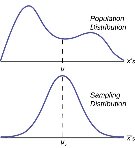
Notice that the horizontal axis in the top panel is labeled X. These are the individual observations of the population. This is the unknown distribution of the population values. The graph is purposefully drawn all squiggly to show that it does not matter just how odd ball it really is. Remember, we will never know what this distribution looks like, or its mean or standard deviation for that matter.

The horizontal axis in the bottom panel is labeled X– ‘s. This is the theoretical distribution called the sampling distribution of the means. Each observation on this distribution is a sample mean. All these sample means were calculated from individual samples with the same sample size. The theoretical sampling distribution contains all of the sample mean values from all the possible samples that could have been taken from the population. Of course, no one would ever actually take all of these samples, but if they did this is how they would look. And the Central Limit Theorem says that they will be normally distributed.

The Central Limit Theorem goes even further and tells us the mean and standard deviation of this theoretical distribution.

Table 7.1

The practical significance of The Central Limit Theorem is that now we can compute probabilities for drawing a sample

mean, X– , in just the same way as we did for drawing specific observations, X’s, when we knew the population mean and standard deviation and that the population data were normally distributed.. The standardizing formula has to be amended to recognize that the mean and standard deviation of the sampling distribution, sometimes, called the standard error of the mean, are different from those of the population distribution, but otherwise nothing has changed. The new standardizing formula is

X– − µ X–

Z =σ X–=

X– – µ

σ n

Notice that µ X– in the first formula has been changed to simply µ in the second version. The reason is that mathematically it can be shown that the expected value of µ X– is equal to µ. This was stated in Table 7.1 above. Mathematically, the E(x) symbol read the “expected value of x”. This formula will be used in the next unit to provide estimates of the unknown population parameter μ.

| Using the Central Limit Theorem

Examples of the Central Limit Theorem

Law of Large Numbers

The law of large numbers says that if you take samples of larger and larger size from any population, then the mean of the

sampling distribution, µ –x

tends to get closer and closer to the true population mean, μ. From the Central Limit Theorem,

we know that as n gets larger and larger, the sample means follow a normal distribution. The larger n gets, the smaller the standard deviation of the sampling distribution gets. (Remember that the standard deviation for the sampling distribution

n
of X– is σ .) This means that the sample mean x– must be closer to the population mean μ as n increases. We can say

that μ is the value that the sample means approach as n gets larger. The Central Limit Theorem illustrates the law of large numbers.

This concept is so important and plays such a critical role in what follows it deserves to be developed further. Indeed, there are two critical issues that flow from the Central Limit Theorem and the application of the Law of Large numbers to it. These are

• The probability density function of the sampling distribution of means is normally distributed regardless of the underlying distribution of the population observations and
• standard deviation of the sampling distribution decreases as the size of the samples that were used to calculate the means for the sampling distribution increases.

Taking these in order. It would seem counterintuitive that the population may have any distribution and the distribution of means coming from it would be normally distributed. With the use of computers, experiments can be simulated that show the process by which the sampling distribution changes as the sample size is increased. These simulations show visually the results of the mathematical proof of the Central Limit Theorem.

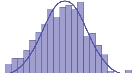
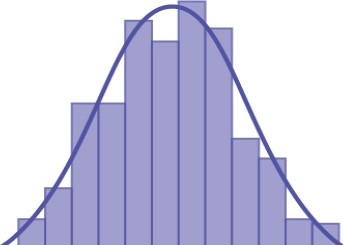
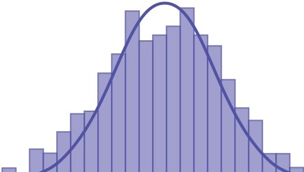
Here are three examples of very different population distributions and the evolution of the sampling distribution to a normal distribution as the sample size increases. The top panel in these cases represents the histogram for the original data. The three panels show the histograms for 1,000 randomly drawn samples for different sample sizes: n=10, n= 25 and n=50. As the sample size increases, and the number of samples taken remains constant, the distribution of the 1,000 sample means becomes closer to the smooth line that represents the normal distribution.

Figure 7.3 is for a normal distribution of individual observations and we would expect the sampling distribution to converge on the normal quickly. The results show this and show that even at a very small sample size the distribution is close to the normal distribution.

This OpenStax book is available for free at http://cnx.org/content/col11776/1.33

Chapter 7 I The Central Limit Theorem311

Normal

20

>-
15

(.) C Q)

0-
=i 10

.Q..).

LL

5

0 X

0246810

Data

Sample Size n = 10

Histogram (with Normal curve) of Mean

70

6050403020
>-

(.)

=ci-

LL

3.03.54.04.55.0

Means

5.56.0

X

6.5

Sample Size n = 25

Histogram (with Normal curve) of Mean

90

80

70

r? 60

50

Q)
5- 40

LL 30

20

10

0 l..d:E:I:Ll ..l..J…LL.Ll..l..l..J…LL.Ll..l…LJt:fX

3.94.04.44.85.2

Means

5.6

6.0

Sample Size n = 50

>- 50(.)40=i0- 30L 2010
Histogram (with Normal c urve) of Mean

L

o Lc:c::c::JU ….L…L..J…J….1…J…..L..J…J…L LIL..J….L:J::z::::c X

3.94 .24.54 .85.15.45.76.0

Means

312Chapter 7 | The Central Limit Theorem

Figure 7.3

Figure 7.4 is a uniform distribution which, a bit amazingly, quickly approached the normal distribution even with only a sample of 10.

This OpenStax book is available for free at http://cnx.org/content/col11776/1.33

Chapter 7 IThe central Limit Theorem313

Distribution of Random Variable

Histogram of Cl

246

Data

X

10-8 —2 -0
810

Sample Size n = 10

Histogram (with Normal curve) of Mean

90

80

70

(>’ 60

50

Q)
6- 40

LL 30

20

10

o L.c:1!!!!!!:::C::::U..LU. .LJU. .LJU. ..LJU. ..LJ…J…..LJ…J….::C=:!!!s=·x

3 .24.04.85 . 66.4

Means

7.28.0

Sample Size n = 25

Histogram (with Normal Curve) of Mean

90

80

70

(>’ 60

C

Q) 50

6- 40

LL 30

20

10

o l.c::l:l!!l;c:[:U .Ll.Ll.L.lLl …LJ..LI..LI..LI..LLI.Dt=·x

4. 04 . 55 .05.56 . 0

Means

6.57.0

Sample Size n = 50

Histogram (with Normal curve) of Mean

10080(,’60,f_il° 40LL20:::J

4.44.85.25.66.0

Means

6.46.8

314Chapter 7 | The Central Limit Theorem

Figure 7.4

Figure 7.5 is a skewed distribution. This last one could be an exponential, geometric, or binomial with a small probability of success creating the skew in the distribution. For skewed distributions our intuition would say that this will take larger sample sizes to move to a normal distribution and indeed that is what we observe from the simulation. Nevertheless, at a sample size of 50, not considered a very large sample, the distribution of sample means has very decidedly gained the shape of the normal distribution.

This OpenStax book is available for free at http://cnx.org/content/col11776/1.33

Chapter 7 IThe Central Limit Theorem315

35

30

>, 25

(.)

20

f::iil”

,…_ 1 5

U. 1 0 5

0

0

481 216

Data

202428

Distribution of Sample means with n = 10

Histogram (with Normal curve) of Mean

160

140120Gl.OOC80fil° 60LL 40
o b::::c::::L.. D….LU.…LL.l..LJLJ..... U….I::r::t– – == x

-0.01.6

3.24.86.48.09.6

Means

Distribution of Sample means with n = 25

Histogram (with Normal Curve) of Mean

100>.80(.)60f,..i.l_” 40l.20::i
L

1.62.43 .24.04.85.66.4

Means Distribution of Sample means with n = 50

Histogram (with Normal c urve) of Mean

g>.

0-

Ll.

8

7

6

5

4

3

2

1
b!!/:td…WWJ..lililWW J..lililW[D3;;:==z:B!x

2.02.53.03.54.04.55.05.5

Means

Figure 7.5

The Central Limit Theorem provides more than the proof that the sampling distribution of means is normally distributed. It also provides us with the mean and standard deviation of this distribution. Further, as discussed above, the expected value of the mean, µ –x , is equal to the mean of the population of the original data which is what we are interested in estimating

from the sample we took. We have already inserted this conclusion of the Central Limit Theorem into the formula we use for standardizing from the sampling distribution to the standard normal distribution. And finally, the Central Limit Theorem

=
n
has also provided the standard deviation of the sampling distribution, σ –x σ , and this is critical to have to calculate

probabilities of values of the new random variable, x– .

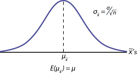
Figure 7.6 shows a sampling distribution. The mean has been marked on the horizontal axis of the x– ‘s and the standard deviation has been written to the right above the distribution. Notice that the standard deviation of the sampling distribution is the original standard deviation of the population, divided by the sample size. We have already seen that as the sample size increases the sampling distribution becomes closer and closer to the normal distribution. As this happens, the standard deviation of the sampling distribution changes in another way; the standard deviation decreases as n increases. At very very large n, the standard deviation of the sampling distribution becomes very small and at infinity it collapses on top of the

population mean. This is what it means that the expected value of µ –x

is the population mean, µ.

Figure 7.6

At non-extreme values of n,this relationship between the standard deviation of the sampling distribution and the sample size plays a very important part in our ability to estimate the parameters we are interested in.

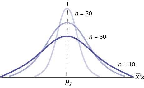
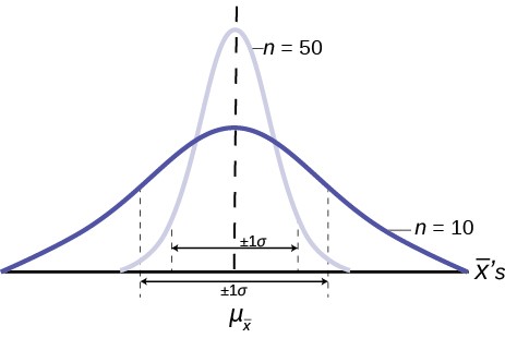
Figure 7.7 shows three sampling distributions. The only change that was made is the sample size that was used to get the sample means for each distribution. As the sample size increases, n goes from 10 to 30 to 50, the standard deviations of the respective sampling distributions decrease because the sample size is in the denominator of the standard deviations of the sampling distributions.

This OpenStax book is available for free at http://cnx.org/content/col11776/1.33

Figure 7.7

The implications for this are very important. Figure 7.8 shows the effect of the sample size on the confidence we will have in our estimates. These are two sampling distributions from the same population. One sampling distribution was created with samples of size 10 and the other with samples of size 50. All other things constant, the sampling distribution with sample size 50 has a smaller standard deviation that causes the graph to be higher and narrower. The important effect of this is that for the same probability of one standard deviation from the mean, this distribution covers much less of a range

of possible values than the other distribution. One standard deviation is marked on the X– axis for each distribution. This

is shown by the two arrows that are plus or minus one standard deviation for each distribution. If the probability that the true mean is one standard deviation away from the mean, then for the sampling distribution with the smaller sample size, the possible range of values is much greater. A simple question is, would you rather have a sample mean from the narrow, tight distribution, or the flat, wide distribution as the estimate of the population mean? Your answer tells us why people intuitively will always choose data from a large sample rather than a small sample. The sample mean they are getting is coming from a more compact distribution. This concept will be the foundation for what will be called level of confidence in the next unit.

Figure 7.8

| The Central Limit Theorem for Proportions

The Central Limit Theorem tells us that the point estimate for the sample mean, x¯ , comes from a normal distribution of x¯ ‘s. This theoretical distribution is called the sampling distribution of x¯ ‘s. We now investigate the sampling distribution for another important parameter we wish to estimate; p from the binomial probability density function.

If the random variable is discrete, such as for categorical data, then the parameter we wish to estimate is the population proportion. This is, of course, the probability of drawing a success in any one random draw. Unlike the case just discussed for a continuous random variable where we did not know the population distribution of X’s, here we actually know the underlying probability density function for these data; it is the binomial. The random variable is X = the number of successes and the parameter we wish to know is p, the probability of drawing a success which is of course the proportion of successes

n
in the population. The question at issue is: from what distribution was the sample proportion, p’ = x drawn? The sample

size is n and X is the number of successes found in that sample. This is a parallel question that was just answered by the Central Limit Theorem: from what distribution was the sample mean, x¯ , drawn? We saw that once we knew that the distribution was the Normal distribution then we were able to create confidence intervals for the population parameter, µ.

We will also use this same information to test hypotheses about the population mean later. We wish now to be able to develop confidence intervals for the population parameter “p” from the binomial probability density function.

In order to find the distribution from which sample proportions come we need to develop the sampling distribution of sample proportions just as we did for sample means. So again imagine that we randomly sample say 50 people and ask them if they support the new school bond issue. From this we find a sample proportion, p’, and graph it on the axis of p’s. We do this again and again etc., etc. until we have the theoretical distribution of p’s. Some sample proportions will show high favorability toward the bond issue and others will show low favorability because random sampling will reflect the variation of views within the population. What we have done can be seen in Figure 7.9. The top panel is the population distributions of probabilities for each possible value of the random variable X. While we do not know what the specific distribution looks like because we do not know p, the population parameter, we do know that it must look something like this. In reality, we do not know either the mean or the standard deviation of this population distribution, the same difficulty we faced when analyzing the X’s previously.

This OpenStax book is available for free at http://cnx.org/content/col11776/1.33

Figure 7.9

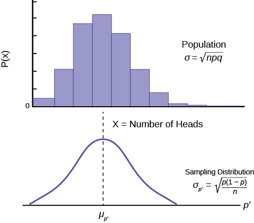
Figure 7.9 places the mean on the distribution of population probabilities as µ = np but of course we do not actually know the population mean because we do not know the population probability of success, p . Below the distribution of the population values is the sampling distribution of p ‘s. Again the Central Limit Theorem tells us that this distribution is normally distributed just like the case of the sampling distribution for x¯ ‘s. This sampling distribution also has a mean, the mean of the p ‘s, and a standard deviation, σp ‘ .

Importantly, in the case of the analysis of the distribution of sample means, the Central Limit Theorem told us the expected value of the mean of the sample means in the sampling distribution, and the standard deviation of the sampling distribution. Again the Central Limit Theorem provides this information for the sampling distribution for proportions. The answers are:

• The expected value of the mean of sampling distribution of sample proportions, µp’ , is the population proportion, p.
• The standard deviation of the sampling distribution of sample proportions, σp’ , is the population standard deviation divided by the square root of the sample size, n.

Both these conclusions are the same as we found for the sampling distribution for sample means. However in this case, because the mean and standard deviation of the binomial distribution both rely upon p , the formula for the standard

deviation of the sampling distribution requires algebraic manipulation to be useful. We will take that up in the next chapter. The proof of these important conclusions from the Central Limit Theorem is provided below.

E(p ‘) = E⎛x⎞ = ⎛1⎞E(x) = ⎛1⎞np = p

⎝n⎠⎝n⎠⎝n⎠

(The expected value of X, E(x), is simply the mean of the binomial distribution which we know to be np.)

⎛ ⎞

p⎛1 − p⎞

σp’2 = Var(p ‘) = Var x = 1 (Var(x)) = 1 (np(1 − p)) = ⎝⎠

⎝n⎠n2n2n

The standard deviation of the sampling distribution for proportions is thus:

p⎛1 − P⎞⎝⎠n
σp’ =

Table 7.2

Table 7.2 summarizes these results and shows the relationship between the population, sample and sampling distribution. Notice the parallel between this Table and Table 7.1 for the case where the random variable is continuous and we were developing the sampling distribution for means.

Reviewing the formula for the standard deviation of the sampling distribution for proportions we see that as n increases the standard deviation decreases. This is the same observation we made for the standard deviation for the sampling distribution for means. Again, as the sample size increases, the point estimate for either µ or p is found to come from a distribution with a narrower and narrower distribution. We concluded that with a given level of probability, the range from which the point estimate comes is smaller as the sample size, n, increases. Figure 7.8 shows this result for the case of sample means. Simply

substitute p ‘ for x¯ and we can see the impact of the sample size on the estimate of the sample proportion.

| Finite Population Correction Factor

x¯− µ σ * N − nnN − 1
We saw that the sample size has an important effect on the variance and thus the standard deviation of the sampling distribution. Also of interest is the proportion of the total population that has been sampled. We have assumed that the population is extremely large and that we have sampled a small part of the population. As the population becomes smaller and we sample a larger number of observations the sample observations are not independent of each other. To correct for the impact of this, the Finite Correction Factor can be used to adjust the variance of the sampling distribution. It is appropriate when more than 5% of the population is being sampled and the population has a known population size. There are cases when the population is known, and therefore the correction factor must be applied. The issue arises for both the sampling distribution of the means and the sampling distribution of proportions. The Finite Population Correction Factor for the variance of the means shown in the standardizing formula is:

Z =

and for the variance of proportions is:

×
−
p⎛1 − p⎞

σp’ =

⎝⎠Nn

nN − 1

The following examples show how to apply the factor. Sampling variances get adjusted using the above formula.

Example 7.1It is learned that the population of White German Shepherds in the USA is 4,000 dogs, and the mean weight for German Shepherds is 75.45 pounds. It is also learned that the population standard deviation is 10.37 pounds.If the sample size is 100 dogs, then find the probability that a sample will have a mean that differs from the true probability mean by less than 2 pounds.

This OpenStax book is available for free at http://cnx.org/content/col11776/1.33

Solution 7.1

N = 4000,n = 100,σ = 10.37,µ = 75.45,⎛ x¯ − µ⎞ = ± 2

⎝⎠

x¯− µ σ * N − nnN − 1

Z == ±2= ± 1.95

10.37 * 4000 − 100

1004000 − 1

⎝
⎠
f ⎛Z⎞ = 0.4744 * 2 = 0.9488

Note that “differs by less” references the area on both sides of the mean within 2 pounds right or left.

Example 7.2When a customer places an order with Rudy’s On-Line Office Supplies, a computerized accounting information system (AIS) automatically checks to see if the customer has exceeded his or her credit limit. Past records indicate that the probability of customers exceeding their credit limit is .06.Suppose that on a given day, 3,000 orders are placed in total. If we randomly select 360 orders, what is the probability that between 10 and 20 customers will exceed their credit limit?Solution 7.2N = 3000, n = 360, p = 0.06σ =p’p 1 − p⎛⎞⎝⎠n× N − 1 =N − n0.06(1 − 0.06)× = 0.01173000 − 360p1 = 10360= 0.0278,360p2 = 203603000 − 1= 0.0556Z =p ‘ − pp⎝1 − p⎞⎛= 0.0278 − 0.06 = −2.74n⎠* N − nN − 10.011744Z =p ‘ − pp⎝1 − p⎞⎛ = 0.0556 − 0.06 = −0.38n⎠*N − n0.011744p⎛0.0278 − 0.06 ∠ z ∠ 0.0556 − 0.06⎞ = p⎛−2.74 ∠ z ∠ −0.38⎞ = 0.4969 − 0.1480 = 0.3489N − 1⎝0.0117440.011744⎠⎝⎠

KEY TERMS

Average a number that describes the central tendency of the data; there are a number of specialized averages, including the arithmetic mean, weighted mean, median, mode, and geometric mean.

–
Central Limit Theorem Given a random variable with known mean μ and known standard deviation, σ, we are sampling with size n, and we are interested in two new RVs: the sample mean, X . If the size (n) of the sample is

n
sufficiently large, then X– ~ N(μ, σ ). If the size (n) of the sample is sufficiently large, then the distribution of the

sample means will approximate a normal distributions regardless of the shape of the population. The mean of the

n
sample means will equal the population mean. The standard deviation of the distribution of the sample means, σ ,

is called the standard error of the mean.

Finite Population Correction Factor adjusts the variance of the sampling distribution if the population is known and more than 5% of the population is being sampled.

–
Mean a number that measures the central tendency; a common name for mean is “average.” The term “mean” is a shortened form of “arithmetic mean.” By definition, the mean for a sample (denoted byx ) is

Number of values in the sample
–x = Sum of all values in the sample ,andthemeanforapopulation(denotedbyμ)is

µ =.
Sum of all values in the population Number of values in the population

Normal Distribution

a continuous random variable with pdf f (x) = 1

σ 2π

– (x – µ)2

e2σ 2, where μ is the mean of the

distribution and σ is the standard deviation.; notation: X ~ N(μ, σ). If μ = 0 and σ = 1, the random variable, Z, is called the standard normal distribution.

Sampling Distribution Given simple random samples of size n from a given population with a measured characteristic such as mean, proportion, or standard deviation for each sample, the probability distribution of all the measured characteristics is called a sampling distribution.

n
Standard Error of the Mean the standard deviation of the distribution of the sample means, or σ .

Standard Error of the Proportion the standard deviation of the sampling distribution of proportions

CHAPTER REVIEW

The Central Limit Theorem for Sample Means

In a population whose distribution may be known or unknown, if the size (n) of samples is sufficiently large, the distribution of the sample means will be approximately normal. The mean of the sample means will equal the population mean. The standard deviation of the distribution of the sample means, called the standard error of the mean, is equal to the population standard deviation divided by the square root of the sample size (n).

Using the Central Limit Theorem

The Central Limit Theorem can be used to illustrate the law of large numbers. The law of large numbers states that the larger the sample size you take from a population, the closer the sample mean x– gets to μ.

The Central Limit Theorem for Proportions

p⎛1 − p⎞⎝⎠n
The Central Limit Theorem can also be used to illustrate that the sampling distribution of sample proportions is normally

distributed with the expected value of p and a standard deviation of σp’ =

This OpenStax book is available for free at http://cnx.org/content/col11776/1.33

FORMULA REVIEW

The Central Limit Theorem for Sample Means

The Central Limit Theorem for Sample Means:

X– ~ N ⎛µ – , σ ⎞

Standard Error of the Mean (Standard Deviation ( X– )):

σ n

x¯− µ σ * N − nnN − 1
Finite Population Correction Factor for the sampling

distribution of means: Z =

p(1 − p)n
N − nN − 1
⎝ xn⎠

X– − µ ––

=
X
Z =σ X–

X – µ σ /n

Finite Population Correction Factor for the sampling

The Mean X– : µ –x

Central Limit Theorem for Sample Means z-score

⎛ σ ⎞
z = x– − µ –x

⎝ n⎠

distribution of proportions: σp’ =×

PRACTICE

Using the Central Limit Theorem

Use the following information to answer the next ten exercises: A manufacturer produces 25-pound lifting weights. The lowest actual weight is 24 pounds, and the highest is 26 pounds. Each weight is equally likely so the distribution of weights is uniform. A sample of 100 weights is taken.

1.

• What is the distribution for the weights of one 25-pound lifting weight? What is the mean and standard deivation?
• What is the distribution for the mean weight of 100 25-pound lifting weights?
• Find the probability that the mean actual weight for the 100 weights is less than 24.9.
• Draw the graph from Exercise 7.1
• Find the probability that the mean actual weight for the 100 weights is greater than 25.2.
• Draw the graph from Exercise 7.3
• Find the 90th percentile for the mean weight for the 100 weights.
• Draw the graph from Exercise 7.5 7.
• What is the distribution for the sum of the weights of 100 25-pound lifting weights? b. Find P(Σx < 2,450).
• Draw the graph from Exercise 7.7
• Find the 90th percentile for the total weight of the 100 weights.
• Draw the graph from Exercise 7.9

Use the following information to answer the next five exercises: The length of time a particular smartphone’s battery lasts follows an exponential distribution with a mean of ten months. A sample of 64 of these smartphones is taken.

• What is the standard deviation?
• What is the parameter m?
• What is the distribution for the length of time one battery lasts?

• What is the distribution for the mean length of time 64 batteries last?
• What is the distribution for the total length of time 64 batteries last?
• Find the probability that the sample mean is between seven and 11.
• Find the 80th percentile for the total length of time 64 batteries last.
• Find the IQR for the mean amount of time 64 batteries last.
• Find the middle 80% for the total amount of time 64 batteries last.

Use the following information to answer the next eight exercises: A uniform distribution has a minimum of six and a maximum of ten. A sample of 50 is taken.

19. Find P(Σx > 420).

• Find the 90th percentile for the sums.
• Find the 15th percentile for the sums.
• Find the first quartile for the sums.
• Find the third quartile for the sums.
• Find the 80th percentile for the sums.
• A population has a mean of 25 and a standard deviation of 2. If it is sampled repeatedly with samples of size 49, what is the mean and standard deviation of the sample means?
• A population has a mean of 48 and a standard deviation of 5. If it is sampled repeatedly with samples of size 36, what is the mean and standard deviation of the sample means?
• A population has a mean of 90 and a standard deviation of 6. If it is sampled repeatedly with samples of size 64, what is the mean and standard deviation of the sample means?
• A population has a mean of 120 and a standard deviation of 2.4. If it is sampled repeatedly with samples of size 40, what is the mean and standard deviation of the sample means?
• A population has a mean of 17 and a standard deviation of 1.2. If it is sampled repeatedly with samples of size 50, what is the mean and standard deviation of the sample means?
• A population has a mean of 17 and a standard deviation of 0.2. If it is sampled repeatedly with samples of size 16, what is the expected value and standard deviation of the sample means?
• A population has a mean of 38 and a standard deviation of 3. If it is sampled repeatedly with samples of size 48, what is the expected value and standard deviation of the sample means?
• A population has a mean of 14 and a standard deviation of 5. If it is sampled repeatedly with samples of size 60, what is the expected value and standard deviation of the sample means?

The Central Limit Theorem for Proportions

• A question is asked of a class of 200 freshmen, and 23% of the students know the correct answer. If a sample of 50 students is taken repeatedly, what is the expected value of the mean of the sampling distribution of sample proportions?
• A question is asked of a class of 200 freshmen, and 23% of the students know the correct answer. If a sample of 50 students is taken repeatedly, what is the standard deviation of the mean of the sampling distribution of sample proportions?
• A game is played repeatedly. A player wins one-fifth of the time. If samples of 40 times the game is played are taken repeatedly, what is the expected value of the mean of the sampling distribution of sample proportions?
• A game is played repeatedly. A player wins one-fifth of the time. If samples of 40 times the game is played are taken repeatedly, what is the standard deviation of the mean of the sampling distribution of sample proportions?
• A virus attacks one in three of the people exposed to it. An entire large city is exposed. If samples of 70 people are taken, what is the expected value of the mean of the sampling distribution of sample proportions?
• A virus attacks one in three of the people exposed to it. An entire large city is exposed. If samples of 70 people are taken, what is the standard deviation of the mean of the sampling distribution of sample proportions?

This OpenStax book is available for free at http://cnx.org/content/col11776/1.33

• A company inspects products coming through its production process, and rejects detected products. One-tenth of the items are rejected. If samples of 50 items are taken, what is the expected value of the mean of the sampling distribution of sample proportions?
• A company inspects products coming through its production process, and rejects detected products. One-tenth of the items are rejected. If samples of 50 items are taken, what is the standard deviation of the mean of the sampling distribution of sample proportions?

Finite Population Correction Factor

• A fishing boat has 1,000 fish on board, with an average weight of 120 pounds and a standard deviation of 6.0 pounds. If sample sizes of 50 fish are checked, what is the probability the fish in a sample will have mean weight within 2.8 pounds the true mean of the population?
• An experimental garden has 500 sunflowers plants. The plants are being treated so they grow to unusual heights. The average height is 9.3 feet with a standard deviation of 0.5 foot. If sample sizes of 60 plants are taken, what is the probability the plants in a given sample will have an average height within 0.1 foot of the true mean of the population?
• A company has 800 employees. The average number of workdays between absence for illness is 123 with a standard deviation of 14 days. Samples of 50 employees are examined. What is the probability a sample has a mean of workdays with no absence for illness of at least 124 days?
• Cars pass an automatic speed check device that monitors 2,000 cars on a given day. This population of cars has an average speed of 67 miles per hour with a standard deviation of 2 miles per hour. If samples of 30 cars are taken, what is the probability a given sample will have an average speed within 0.50 mile per hour of the population mean?
• A town keeps weather records. From these records it has been determined that it rains on an average of 37% of the days each year. If 30 days are selected at random from one year, what is the probability that at least 5 and at most 11 days had rain?
• A maker of yardsticks has an ink problem that causes the markings to smear on 4% of the yardsticks. The daily production run is 2,000 yardsticks. What is the probability if a sample of 100 yardsticks is checked, there will be ink smeared on at most 4 yardsticks?
• A school has 300 students. Usually, there are an average of 21 students who are absent. If a sample of 30 students is taken on a certain day, what is the probability that at most 2 students in the sample will be absent?
• A college gives a placement test to 5,000 incoming students each year. On the average 1,213 place in one or more developmental courses. If a sample of 50 is taken from the 5,000, what is the probability at most 12 of those sampled will have to take at least one developmental course?

HOMEWORK

The Central Limit Theorem for Sample Means

• Previously, De Anza statistics students estimated that the amount of change daytime statistics students carry is exponentially distributed with a mean of $0.88. Suppose that we randomly pick 25 daytime statistics students.
• In words, Χ =

b. Χ ~ ( ,)

c. In words, X– =

d.X– ~ ( , )

• Find the probability that an individual had between $0.80 and $1.00. Graph the situation, and shade in the area to be determined.
• Find the probability that the average of the 25 students was between $0.80 and $1.00. Graph the situation, and shade in the area to be determined.
• Explain why there is a difference in part e and part f.

• Suppose that the distance of fly balls hit to the outfield (in baseball) is normally distributed with a mean of 250 feet and a standard dev–iation of 50 feet. We randomly sample 49 fly balls.–
• If X = average distance in feet for 49 fly balls, then X ~ ( ,)
• –
  What is the probability that the 49 balls traveled an average of less than 240 feet? Sketch the graph. Scale the horizontal axis for X . Shade the region corresponding to the probability. Find the probability.
• Find the 80th percentile of the distribution of the average of 49 fly balls.
• According to the Internal Revenue Service, the average length of time for an individual to complete (keep records for, learn, prepare, copy, assemble, and send) IRS Form 1040 is 10.53 hours (without any attached schedules). The distribution is unknown. Let us assume that the standard deviation is two hours. Suppose we randomly sample 36 taxpayers.
• In words, Χ–=
• In words, X =

c.X– ~ ( ,)

• Would you be surprised if the 36 taxpayers finished their Form 1040s in an average of more than 12 hours? Explain why or why not in complete sentences.
• Would you be surprised if one taxpayer finished his or her Form 1040 in more than 12 hours? In a complete sentence, explain why.
• Suppose that a category of world-class runners are known to run a–marathon (26 miles) in an average of 145 minutes

with a standard deviation of 14 minutes. Consider 49 of the races. Let X

a.X– ~ ( ,)

the average of the 49 races.

• Find the probability that the runner will average between 142 and 146 minutes in these 49 marathons.
• Find the 80th percentile for the average of these 49 marathons.
• Find the median of the average running times.
• The length of songs in a collector’s iTunes album collection is uniformly distributed from two to 3.5 minutes. Suppose we randomly pick five albums from the collection. There are a total of 43 songs on the five albums.
• In words, Χ =

b. Χ ~–

c. In words, X =

d.X– ~ ( ,)

• Find the first quartile for the average song length.
• The IQR(interquartile range) for the average song length is from – .
• In 1940 the average size of a U.S. farm was 174 acres. Let’s say that the standard deviation was 55 acres. Suppose we randomly survey 38 farmers from 1940.
• In words, Χ =
• In words, X– =

c.X– ~ ( ,)

d. The IQR for X– is from acres to acres.

• Determine which of the following are true and whi–ch are false. Then, in complete sentences, justify your answers.
• When the sample size is large, the mean of X is approximately equal to the mean of Χ.
• When the sample size is large, X– is approximately normally distributed.
• When the sample size is large, the standard deviation of X– is approximately the same as the standard deviation

of Χ.

• The percent of fat calories that a person in America consumes each day is normally distribut–ed with a mean of about 36

and a standard deviation of about ten. Suppose that 16 individuals are randomly chosen. Let X = average percent of fat

calories.–

X

~ ( , )

• For the group of 16, find the probability that the average percent of fat calories consumed is more than five. Graph the situation and shade in the area to be determined.
• Find the first quartile for the average percent of fat calories.

This OpenStax book is available for free at http://cnx.org/content/col11776/1.33

• The distribution of income in some Third World countries is considered wedge shaped (many very poor people, very few middle income people, and even fewer wealthy people). Suppose we pick a country with a wedge shaped distribution. Let the average salary be $2,000 per year with a standard deviation of $8,000. We randomly survey 1,000 residents of that country.
• In words, Χ =
• In words, X– =

c.X– ~ ( ,)

• How is it possible for the standard deviation to be greater than the average?
• Why is it more likely that the average of the 1,000 residents will be from $2,000 to $2,100 than from $2,100 to

$2,200?

• Which of the following is NOT TRUE about the distribution for averages?
• The mean, median, and mode are equal.
• The area under the curve is one.
• The curve never touches the x-axis.
• The curve is skewed to the right.
• The cost of unleaded gasoline in the Bay Area once followed an unknown distribution with a mean of $4.59 and a standard deviation of $0.10. Sixteen gas stations from the Bay Area are randomly chosen. We are interested in the average cost of gasoline for the 16 gas stations. The distribution to use for the average cost of gasoline for the 16 gas stations is:

a.X– ~ N(4.59, 0.10)

b.X– ~ N ⎛4.59, 0.10⎞

⎝16 ⎠

c.X– ~ N ⎛4.59, 16 ⎞

⎝0.10⎠

d.X– ~ N ⎛4.59, 16 ⎞

⎝0.10⎠

Using the Central Limit Theorem

• A large population of 5,000 students take a practice test to prepare for a standardized test. The population mean is 140 questions correct, and the standard deviation is 80. What size samples should a researcher take to get a distribution of means of the samples with a standard deviation of 10?
• A large population has skewed data with a mean of 70 and a standard deviation of 6. Samples of size 100 are taken, and the distribution of the means of these samples is analyzed.
• Will the distribution of the means be closer to a normal distribution than the distribution of the population?
• Will the mean of the means of the samples remain close to 70?
• Will the distribution of the means have a smaller standard deviation?
• What is that standard deviation?
• A researcher is looking at data from a large population with a standard deviation that is much too large. In order to concentrate the information, the researcher decides to repeatedly sample the data and use the distribution of the means of the samples? The first effort used sample sized of 100. But the standard deviation was about double the value the researcher wanted. What is the smallest size samples the researcher can use to remedy the problem?
• A researcher looks at a large set of data, and concludes the population has a standard deviation of 40. Using sample sizes of 64, the researcher is able to focus the mean of the means of the sample to a narrower distribution where the standard deviation is 5. Then, the researcher realizes there was an error in the original calculations, and the initial standard deviation is really 20. Since the standard deviation of the means of the samples was obtained using the original standard deviation, this value is also impacted by the discovery of the error. What is the correct value of the standard deviation of the means of the samples?
• A population has a standard deviation of 50. It is sampled with samples of size 100. What is the variance of the means of the samples?

The Central Limit Theorem for Proportions

• A farmer picks pumpkins from a large field. The farmer makes samples of 260 pumpkins and inspects them. If one in fifty pumpkins are not fit to market and will be saved for seeds, what is the standard deviation of the mean of the sampling distribution of sample proportions?
• A store surveys customers to see if they are satisfied with the service they received. Samples of 25 surveys are taken. One in five people are unsatisfied. What is the variance of the mean of the sampling distribution of sample proportions for the number of unsatisfied customers? What is the variance for satisfied customers?
• A company gives an anonymous survey to its employees to see what percent of its employees are happy. The company is too large to check each response, so samples of 50 are taken, and the tendency is that three-fourths of the employees are happy. For the mean of the sampling distribution of sample proportions, answer the following questions, if the sample size is doubled.
• How does this affect the mean?
• How does this affect the standard deviation?
• How does this affect the variance?
• A pollster asks a single question with only yes and no as answer possibilities. The poll is conducted nationwide, so samples of 100 responses are taken. There are four yes answers for each no answer overall. For the mean of the sampling distribution of sample proportions, find the following for yes answers.
• The expected value.
• The standard deviation.
• The variance.
• The mean of the sampling distribution of sample proportions has a value of p of 0.3, and sample size of 40.
• Is there a difference in the expected value if p and q reverse roles?
• Is there a difference in the calculation of the standard deviation with the same reversal?

Finite Population Correction Factor

• A company has 1,000 employees. The average number of workdays between absence for illness is 80 with a standard deviation of 11 days. Samples of 80 employees are examined. What is the probability a sample has a mean of workdays with no absence for illness of at least 78 days and at most 84 days?
• Trucks pass an automatic scale that monitors 2,000 trucks. This population of trucks has an average weight of 20 tons with a standard deviation of 2 tons. If a sample of 50 trucks is taken, what is the probability the sample will have an average weight within one-half ton of the population mean?
• A town keeps weather records. From these records it has been determined that it rains on an average of 12% of the days each year. If 30 days are selected at random from one year, what is the probability that at most 3 days had rain?
• A maker of greeting cards has an ink problem that causes the ink to smear on 7% of the cards. The daily production run is 500 cards. What is the probability that if a sample of 35 cards is checked, there will be ink smeared on at most 5 cards?
• A school has 500 students. Usually, there are an average of 20 students who are absent. If a sample of 30 students is taken on a certain day, what is the probability that at least 2 students in the sample will be absent?

REFERENCES

7.1 The Central Limit Theorem for Sample Means

Baran, Daya. “20 Percent of Americans Have Never Used Email.”WebGuild, 2010. Available online at http://www.webguild.org/20080519/20-percent-of-americans-have-never-used-email (accessed May 17, 2013).

Data from The Flurry Blog, 2013. Available online at http://blog.flurry.com (accessed May 17, 2013). Data from the United States Department of Agriculture.

This OpenStax book is available for free at http://cnx.org/content/col11776/1.33

SOLUTIONS

1

a. U(24, 26), 25, 0.5774

b. N(25, 0.0577)

c. 0.0416

3 0.0003

5 25.07

7

a. N(2,500, 5.7735)

• 0

9 2,507.40

11

• 10
• 1 10

13 N ⎛10, 10⎞

⎝8 ⎠

15 0.7799

17 1.69

19 0.0072

21 391.54

23 405.51

• Mean = 25, standard deviation = 2/7
• Mean = 48, standard deviation = 5/6
• Mean = 90, standard deviation = 3/4
• Mean = 120, standard deviation = 0.38
• Mean = 17, standard deviation = 0.17
• Expected value = 17, standard deviation = 0.05
• Expected value = 38, standard deviation = 0.43
• Expected value = 14, standard deviation = 0.65

60 64

61

• Yes
• Yes
• Yes

d. 0.6

62 400

63 2.5

64 25

33 0.23

34 0.060

35 1/5

36 0.063

37 1/3

38 0.056

39 1/10

40 0.042

41 0.999

42 0.901

43 0.301

44 0.832

45 0.483

46 0.500

47 0.502

48 0.519

49

a. Χ = amount of change students carry

b. Χ ~ E(0.88, 0.88)

c.X– = average amount of change carried by a sample of 25 students. d.X– ~ N(0.88, 0.176)

e. 0.0819

f. 0.1882

g. The distributions are different. Part a is exponential and part b is normal.

51

• length of time for an individual to complete IRS form 1040, in hours.
• mean length of time for a sample of 36 taxpayers to complete IRS form 1040, in hours.

c. N ⎛10.53, 1⎞

⎝3⎠

• Yes. I would be surprised, because the probability is almost 0.
• No. I would not be totally surprised because the probability is 0.2312

53

a. the length of a song, in minutes, in the collection b. U(2, 3.5)

c. the average length, in minutes, of the songs from a sample of five albums from the collection d. N(2.75, 0.066)

• 2.74 minutes
• 0.03 minutes

55

• True. The mean of a sampling distribution of the means is approximately the mean of the data distribution.
• True. According to the Central Limit Theorem, the larger the sample, the closer the sampling distribution of the means

This OpenStax book is available for free at http://cnx.org/content/col11776/1.33

becomes normal.

• The standard deviation of the sampling distribution of the means will decrease making it approximately the same as the standard deviation of X as the sample size increases.

57

• X = the yearly income of someone in a third world country
• the average salary from samples of 1,000 residents of a third world country

c.X– ∼ N ⎛2000, 8000 ⎞

⎝1000⎠

• Very wide differences in data values can have averages smaller than standard deviations.
• The distribu–tion of the sample mean will have higher probabilities closer to the population mean.

P(2000 < X < 2100) = 0.1537

P(2100 < X– < 2200) = 0.1317

59 b 60 64 61

• Yes
• Yes
• Yes

d. 0.6

62 400

63 2.5

64 25

65 0.0087

66 0.0064, 0.0064

67

• It has no effect.
• It is divided by 2 .
• It is divided by 2.

68

a. 4/5

b. 0.04

c. 0.0016

69

• Yes
• No

70 0.955

This OpenStax book is available for free at http://cnx.org/content/col11776/1.33